At a million tokens of context, the model’s weights stop being the expensive part. The bill is the key-value (KV) cache, the per-token memory that every attention layer keeps so later tokens can look back, plus the work each new token does to read it. DeepSeek-V3.2 already cut the reading cost: its DeepSeek Sparse Attention (DSA) lets each query read only a small, selected set of past tokens. But it still cached an entry for every token in every layer.

DeepSeek-V4 goes after the other half of the bill. It shrinks the cache along the sequence axis. A small learned compressor turns every 4 tokens, or every 128 tokens, into one 512-number entry, and attention reads those entries instead of raw tokens. Every layer also keeps uncompressed keys and values for the most recent 128 tokens. No main layer in V4 attends densely over all raw tokens.

The payoff, in DeepSeek’s own numbers: at a 1M-token context, DeepSeek-V4-Pro needs 27% of DeepSeek-V3.2’s single-token inference FLOPs (estimated, in equivalent FP8 FLOPs) and 10% of its KV cache, even though it activates more parameters per token. The smaller DeepSeek-V4-Flash needs 10% of the FLOPs and 7% of the cache. Pro has 1.6T parameters (49B active per token); Flash has 284B (13B active).

This post takes both models apart layer by layer. It is built from public sources, and it says which source each claim comes from:

• Paper: the DeepSeek-V4 technical report, “DeepSeek-V4: Towards Highly Efficient Million-Token Context Intelligence” (arXiv 2606.19348; the abstract page says it was submitted on April 26, 2026).
• Configs and model cards: the Hugging Face repos of V4-Pro and V4-Flash, the later releases V4-Pro-DSpark, V4-Flash-0731, V4-Pro-0813, and V4-Flash-Vision-Exp, and the successor DeepSeek-V4.1-Flash.
• Code: DeepSeek’s official reference inference code that ships in the repos (inference/model.py and kernel.py). The model.py files of Pro and Flash are identical; only the configs differ.
• A second report: the DeepSeek-V4.1-Flash technical report, shipped as a PDF in its repo.
• Training code: the open DeepSeek-V4 implementation in Miles, which we covered in the Miles v0.1 deep dive.

When the paper and the code disagree, we say so. Numbers we computed ourselves from the configs, such as parameter breakdowns and cache sizes, are marked “derived.” Our readings of the evidence are marked as interpretation. Where the sources are silent, we say that too, and §14 collects those gaps.

You should know what a large language model (LLM), attention, and a transformer layer are. V4 also builds on ideas we already explained in the GLM-5.3 deep dive: Multi-head Latent Attention (MLA, its §3), the mixture-of-experts (MoE) router with bias-based load balancing (§4.3), DSA and its lightning indexer (§5.1–5.4), and manifold-constrained hyper-connections (mHC, §8.6). We recap each in a sentence or two and spend our time on what V4 does differently.

The sections build on each other:

• §1: the family at a glance: from V3.2 to the V4 previews and the later releases, and a side-by-side table of Pro and Flash.
• §2: a tour of V4’s layers: the path of one token, the per-layer schedule of attention types, and where the parameters live (3D model: the layer stack).
• §3: the attention core: one 512-number vector per token that serves as both key and value for every query head, partial rotary position embedding (RoPE) with a rotation undone on the output, and a grouped output projection (3D model: shared-KV attention).
• §4: the KV compressor: learned, per-channel pooling of 4 or 128 tokens into one entry (3D model: the compressor).
• §5: Compressed Sparse Attention (CSA): a lightning indexer picks the best compressed entries (3D model: one CSA query).
• §6: Heavily Compressed Attention (HCA): compress 128 to 1, then read everything, and why V4 alternates the two (3D model: HCA vs CSA).
• §7: mHC: four residual streams mixed by a doubly stochastic matrix (3D model: the streams).
• §8: the MoE layers: 384 or 256 experts, 6 per token, hash routing in the first three layers, and FP4 experts (3D model: the expert city).
• §9: long context: positions up to 1M, the KV cache and per-token compute against V3.2, and how serving handles a mixed cache (3D model: cache scaling).
• §10: training: data, the Muon optimizer, stability tricks, and FP4 quantization-aware training (applied during post-training).
• §11: post-training and the three reasoning modes.
• §12: after the preview: the speculative-decoding module, the official 0731 and 0813 releases, a vision model, and V4.1-Flash’s new design.
• §13: training notes from the open Miles implementation.
• §14: open questions the sources do not settle.

---

1. The Family at a Glance

Where do V4-Pro and V4-Flash come from, and how do the two differ? This section places them on DeepSeek’s timeline and lines them up in one table. The short version: one architecture, two sizes, and a string of later releases that kept the skeleton, added a drafter, and changed the training.

1.1 From V3.2 to V4, and the releases that followed

V4 inherits two things from DeepSeek-V3: the DeepSeekMoE expert layout and multi-token prediction (MTP), according to the report. From DeepSeek-V3.2 it takes the lightning indexer of DSA and reuses it inside one of its two new attention types. Most of the rest of the attention path is new (the low-rank query projection is the one MLA piece it keeps), and so is the residual connection. The animation below traces the family.

DeepSeek-V4 forks from V3.2 into Pro and Flash previews; DSpark and the official 0731/0813 releases keep the same backbone while agentic scores jump. V4.1-Flash is a separate, new architecture (CSA2, FP4 KV, Engram). Open the full-size SVG.

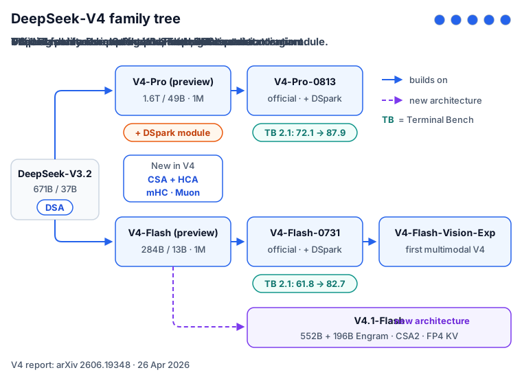
Model	What it is	Total / active parameters
DeepSeek-V3.2	the predecessor: MLA with DSA	671B / 37B
DeepSeek-V4-Pro (preview)	new architecture, 61 layers + 1 MTP layer, 1M context	1.6T / 49B
DeepSeek-V4-Flash (preview)	same architecture, 43 layers + 1 MTP layer, 1M context	284B / 13B
DeepSeek-V4-Pro-DSpark	“not a new model”: the Pro checkpoint plus a speculative-decoding module	same as Pro
DeepSeek-V4-Flash-0731	the official Flash, “superseding the preview version”; same structure as V4-Flash-DSpark	same as Flash
DeepSeek-V4-Pro-0813	the official Pro, built on the preview structure with the DSpark module attached	same as Pro
DeepSeek-V4-Flash-Vision-Exp	“first experimental multimodal model in the DeepSeek-V4 family”: V4-Flash plus visual modules and continued training	not stated
DeepSeek-V4.1-Flash	a new architecture with Engram memory (a large token n-gram lookup table, §12.4)	552B backbone + 196B Engram memory; 16B active in decoding, 8B in prefill

The rows follow the order the cards imply: each later card builds on, or compares against, the ones above it. Three facts about the family matter for the rest of the post:

• One skeleton. The preview Pro and Flash share one architecture and one reference implementation. Only the sizes differ (§1.2).
• The skeleton stayed fixed. DSpark, 0731, 0813, and Vision-Exp keep the preview’s text backbone. Speed comes from a speculative-decoding module, quality gains from new post-training, and Vision-Exp adds visual modules with continued training (§12.1–12.3).
• V4.1-Flash is the real successor. It rethinks the attention design and is a different, larger model (§12.4).

All the model cards we read carry the MIT license.

Dates and names

• The only date we can verify from the sources is the report’s: its arXiv abstract page says “Submitted on 26 Apr 2026,” and only version 1 is listed. Its identifier, 2606.19348, would normally point to a June 2026 submission. We flag the mismatch and do not try to resolve it.
• None of the model cards states a release date, so the table gives none. The suffixes -0731 and -0813 suggest July 31 and August 13 (month-day naming); that is our reading, and the cards do not spell it out.
• The 0731 card describes V4-Flash-0731 as having “the same model structure as DeepSeek-V4-Flash-DSpark.” We did not read a V4-Flash-DSpark repo; only V4-Pro-DSpark is among our sources.
• The V3.2 row’s parameter counts come from the “# Activated Params” and “# Total Params” rows of the base-model table in the V4 cards (37B and 671B).

1.2 Pro and Flash side by side

Pro and Flash share every design choice: the attention types, the 512-wide heads, the 128-token window, the residual streams, and the router. They differ in width, depth, and expert count, plus one detail in the first two layers:

	DeepSeek-V4-Pro	DeepSeek-V4-Flash
Total / active parameters	1.6T / 49B	284B / 13B
Pre-training tokens	33T	32T
Layers	61 (+1 MTP)	43 (+1 MTP)
Hidden size	7,168	4,096
Query heads × head dimension	128 × 512	64 × 512
KV heads	1 (shared by all query heads)	1
Query low-rank width	1,536	1,024
Output projection	16 groups, each to 1,024	8 groups, each to 1,024
Sliding window (every layer)	128 tokens	128 tokens
Compression ratios	4 (CSA) and 128 (HCA)	4 (CSA) and 128 (HCA)
Attention layer mix	30 CSA + 31 HCA	21 CSA + 20 HCA + 2 window-only
Layers 0–1	HCA	sliding window only
Indexer heads × dim / entries kept	64 × 128 / 1,024	64 × 128 / 512
Experts per layer	384 routed + 1 shared, top-6	256 routed + 1 shared, top-6
Expert inner width	3,072	2,048
Routing scale	2.5	1.5
Hash-routed layers	0–2	0–2
Residual streams (mHC)	4, 20 Sinkhorn iterations	4, 20 Sinkhorn iterations
Vocabulary / max positions	129,280 / 1,048,576	129,280 / 1,048,576

A few terms in the table get a short definition now and a full section later. A sliding window keeps uncompressed keys and values for the most recent 128 tokens. A compression ratio of 4 means the cache holds one entry per four consecutive tokens (§4). CSA layers pick a fixed number of those entries with an indexer (§5); HCA layers fold 128 tokens per entry and read all of them (§6). Hash-routed layers pick experts from a fixed table indexed by token ID (§8.3).

Both models activate a small share of their weights per token: 3.06% for Pro and 4.58% for Flash, against 5.51% for V3.2 (derived from the published totals). Pro is the sparser model even though it is far larger.

Where the numbers come from

• Every structural row comes from the two config.json files (keys such as num_hidden_layers, hidden_size, num_attention_heads, head_dim, num_key_value_heads, q_lora_rank, o_groups, o_lora_rank, sliding_window, index_n_heads, index_head_dim, index_topk, n_routed_experts, moe_intermediate_size, routed_scaling_factor, num_hash_layers, hc_mult, hc_sinkhorn_iters). The report’s model-setup section (§4.2.1) restates the structural values (layers, hidden size, heads, head dim, query compression, output groups, window, indexer, experts, hash layers, mHC), and every value it gives matches the configs. The routing scale, KV-head count, vocabulary and max positions come from the configs only.
• The layer mix comes from the per-layer list compress_ratios (62 entries for Pro, 44 for Flash: one per main layer plus one for the MTP layer); §2.2 decodes it. The report says the same in words. For Flash: “For the first two layers, we use pure sliding window attention.” For Pro: “For the first two layers, we use HCA.”
• The totals (1.6T / 49B and 284B / 13B) are the report’s and the cards’; the token counts (33T for Pro, 32T for Flash) are the report’s. The cards say “more than 32T” for both.
• The activation shares divide active by total parameters: 49 / 1,600, 13 / 284, and 37 / 671.

How do the base models (before post-training) compare with V3.2’s? A few rows from the cards’ base-model table:

Benchmark (shots)	V3.2-Base	V4-Flash-Base	V4-Pro-Base
MMLU-Pro (5)	65.5	68.3	73.5
Simple-QA verified (25)	28.3	30.1	55.2
FACTS Parametric (25)	27.1	33.9	62.6
HumanEval (0)	62.8	69.5	76.8
LongBench-V2 (1)	40.2	44.7	51.5
BBH (3)	87.6	86.9	87.5
BigCodeBench (3)	63.9	56.8	59.2
MATH (4)	60.5	57.4	64.5

Pro-Base leads on most rows, and by far on the knowledge tests (Simple-QA verified nearly doubles V3.2-Base’s score, and FACTS Parametric more than doubles it). Flash-Base, with about a third of V3.2’s active parameters, beats V3.2-Base on most rows but not all. It trails on 7 of the card’s 25 benchmark rows, most clearly BigCodeBench (56.8 vs 63.9) and MATH (57.4 vs 60.5); V3.2-Base also stays ahead of both V4 bases on BigCodeBench and BBH (87.6 vs 86.9 / 87.5).

1.3 Two stories in one family

The rest of the post follows a simple split. The first story is the preview architecture (§2–§11): how V4 compresses attention, widens the residual stream, routes tokens to experts, and how DeepSeek trained it. Everything there applies to both Pro and Flash, with their own numbers.

The second story is what came after (§12). The official 0731 and 0813 releases kept the backbone’s weight shapes, attached a speculative-decoding module, and gained mostly from agentic post-training. V4.1-Flash then rethought the attention design and pushed KV compression further.

2. A Tour of V4’s Layers

What happens to one token on its way through V4? It climbs a stack of layers that all share one shape: an attention block, then an MoE block, each wrapped in a widened residual connection. The layers differ mainly in one way: the kind of memory their attention reads, and this section shows which layer reads what.

2.1 The path of a token

Here is the trip through V4-Pro, with Flash’s sizes in parentheses. “Hidden state” means the vector of numbers that represents the token between layers.

1. Embedding. The token’s ID picks one row of a 129,280 × 7,168 table (× 4,096 for Flash).
2. Four streams. The vector is copied four times. From here on, each token carries a residual of 4 × 7,168 numbers instead of one vector. This is mHC (§7).
3. Attention sublayer. A small learned mix collapses the 4 streams into one input. Then come RMSNorm (a scale normalization), attention, and a learned write-back into all 4 streams.
4. MoE sublayer. The same pattern again: mix 4 streams into one, RMSNorm, then an MoE layer with 384 routed experts (256) plus 1 shared expert, of which each token uses 6 routed experts plus the shared one. Then write back.
5. Repeat steps 3–4 for all 61 layers (43).
6. Output. A final sigmoid-weighted mix turns the 4 streams into one vector, then RMSNorm and an output projection (lm_head) to 129,280 vocabulary scores. The output projection does not reuse the embedding table.
7. MTP layer. One extra layer with its own attention and MoE predicts one further token and adds an MTP loss during training. The report keeps V3’s MTP configuration unchanged.

Two things are missing from this list compared with V3-style models. There are no dense feed-forward layers: every layer, including the first, is MoE. And there is no layer whose attention reads every past token at full resolution.

Implementation notes

• In model.py, Transformer.forward embeds the tokens and repeats them along a new stream axis (h.unsqueeze(2).repeat(1, 1, hc_mult, 1), hc_mult = 4). Each Block.forward runs hc_pre → attn_norm → attn → hc_post, then hc_pre → ffn_norm → ffn → hc_post, with separate mixing weights for the two sublayers.
• The final collapse is ParallelHead.hc_head: sigmoid weights over the 4 streams, with no Sinkhorn step. Logits are computed for the last position only at inference.
• The MTP block (MTPBlock) reuses the main model’s embedding and lm_head. It normalizes the token embedding and the incoming hidden state separately (enorm, hnorm), projects each with its own 7,168 × 7,168 matrix (e_proj, h_proj), adds them, and then runs an ordinary Block. It has its own stream collapse (hc_head_fn).
• Block always builds an MoE; there is no first_k_dense_replace-style switch. The report confirms: “We employ MoE layers in all Transformer blocks.”

Inside the attention sublayer, every V4 layer does the same thing. It builds one list of keys and runs one softmax over it. The list always starts with the raw keys of the last 128 tokens, the sliding window. What follows depends on the layer type:

• CSA layer (ratio 4): the window plus the compressed entries (one per 4 tokens) that a lightning indexer ranks highest: at most 1,024 in Pro and 512 in Flash.
• HCA layer (ratio 128): the window plus every completed compressed entry (one per 128 tokens).
• Window-only layer: just the 128 window keys.

Each head also has a learned “sink” logit that joins the softmax’s denominator, so a head can put weight on nothing at all (§3.4). The animation below shows the two compressed lanes and the window feeding that single softmax.

Every V4 attention layer reads the last 128 tokens exactly plus one compressed lane: CSA (4 tokens per entry, indexer keeps top-k) or HCA (128 tokens per entry, all read). Both parts share one softmax with a learned sink over a single 512-d KV head, and the two layer types alternate. Open the full-size SVG.

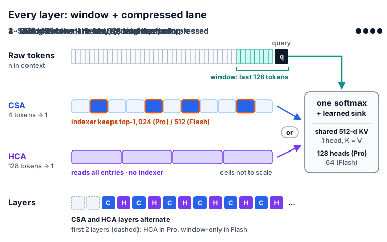
A tiny example makes the list concrete. Take a query at position 10,000 in a Pro CSA layer. The window covers positions 9,873 to 10,000. Positions 0 to 9,999 form 2,500 completed 4-token blocks, so the indexer ranks 2,500 compressed entries and keeps the top 1,024. The softmax runs over 128 + 1,024 = 1,152 keys. In an HCA layer, the same query sees 78 completed 128-token entries (78 × 128 = 9,984) plus the window: 206 keys (all counts derived from the code’s rules).

Every key in the list is the same kind of object: one 512-number vector that serves as both key and value for all query heads. Raw window tokens and compressed entries live in the same 512-dimensional space, so a single kernel can attend over both. §3 explains that vector, and §4 explains how compressed entries are made.

Implementation notes

• In Attention.forward, the window indices come from get_window_topk_idxs (the last 128 positions, including the query’s own). A CSA layer appends the indexer’s top-k (min(index_topk, completed entries)); an HCA layer appends all completed entries (get_compress_topk_idxs). Both lists go to one sparse_attn call with the per-head attn_sink.
• A compressed entry for block $j$ becomes visible only once the block is complete, that is, when the query position $s$ satisfies $s \ge jr + r - 1$ for ratio $r$. In the example, position 10,000 starts a new 4-token block (10,000 = 4 × 2,500), so the query sees blocks 0 to 2,499; the window holds its own token.
• There is no gate or second softmax that balances the window against the compressed part. Both compete inside the same softmax.

2.2 The layer schedule

Which layers are CSA, which are HCA, and which are window-only? The config answers with one list, compress_ratios, that holds one number per layer: 4 for CSA, 128 for HCA, and 0 for window-only. Its last entry belongs to the MTP layer. Here is how the two lists read, layer by layer:

Layer	0	1	2	3	4	5	…	last main layer	MTP
Pro	128	128	4	128	4	128	…	4 (layer 60)	0
Flash	0	0	4	128	4	128	…	4 (layer 42)	0

From layer 2 on, both models alternate: even layers are CSA and odd layers are HCA, ending on a CSA layer. Counting it out:

• Pro (61 layers): layers 0–1 are HCA. Layers 2–60 hold 30 CSA layers (2, 4, …, 60) and 29 HCA layers (3, 5, …, 59). Total: 30 CSA + 31 HCA, and no window-only main layer.
• Flash (43 layers): layers 0–1 are window-only. Layers 2–42 hold 21 CSA layers (2, 4, …, 42) and 20 HCA layers (3, 5, …, 41). Total: 21 CSA + 20 HCA + 2 window-only.
• MTP layer (both): window-only.

Two more per-layer switches ride on the same index. The MoE in layers 0, 1, and 2 uses hash routing: a fixed table maps each token ID to its 6 experts (§8.3). And RoPE changes with the layer type. Compressed layers use a RoPE base of 160,000 with YaRN (a method that stretches RoPE to longer contexts) scaling to reach 1M positions; window-only layers use base 10,000 and no YaRN (§9.1). The paper text does not discuss YaRN; this comes from the config and code.

The 3D model below stacks both schedules side by side; hover a layer for its type, its RoPE setting, and how many keys one query reads at a chosen context length.

DeepSeek-V4-Pro (61 layers) and V4-Flash (43 layers) layer by layer: every layer keeps an exact 128-token window (cyan core) and adds either CSA top-k (blue, ratio 4), all HCA entries (teal, ratio 128) or nothing (grey, Flash layers 0-1 and the MTP layer); there is no dense full-attention layer. Slab width shows log2 of the keys each query reads at the chosen context (illustrative); layer counts, types, hash layers 0-2 and the exact key counts in the panel come from the configs and DeepSeek's reference code.

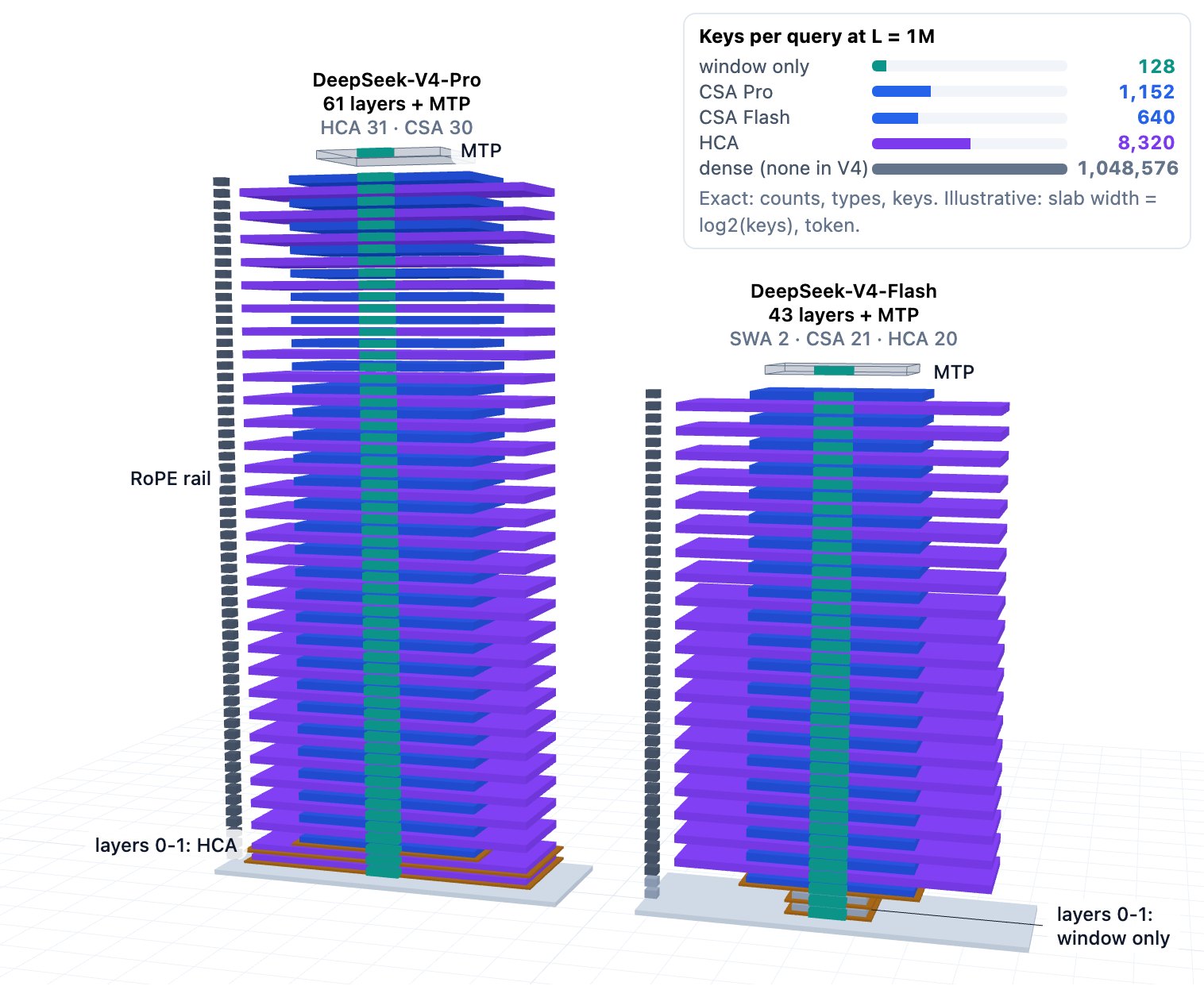
So there is no dense full-attention layer anywhere in V4. Every main layer reads the 128-token window, and all but Flash’s first two also read a compressed memory.

Implementation notes

• The lists have 62 entries (Pro) and 44 (Flash). The MTP block is built with layer_id = n_layers + i, so it reads the final entry, which is 0 in both.
• An Attention with ratio 0 builds no compressor, keeps a KV cache of exactly 128 slots, and sets original_seq_len = 0 so YaRN is off (“disable YaRN and use base rope_theta in pure sliding-window attention,” says the code comment). Compressed layers share one RoPE table across attention, compressor, and indexer.
• The later configs (DSpark, 0731, 0813, Vision-Exp) have two more entries: 64 for Pro, 46 for Flash, all trailing 0s. They also add dspark_block_size: 5 and dspark_target_layer_ids ([58, 59, 60] for Pro, [40, 41, 42] for Flash). Our reading is that the extra entries index the speculative-decoding module’s own window-only blocks; the configs do not label them (§12.1).

2.3 Where the parameters live

Nearly all of V4’s weights sit in the routed experts, and any one token touches only 6 of them per layer. The breakdown below is our own count from the config shapes; the official totals are 1.6T / 49B (Pro) and 284B / 13B (Flash).

Component (derived from the configs)	Pro	Flash
Attention core (query, KV, and output projections), all layers	18.3B (299.9M per layer)	4.6B (107.0M per layer)
Compressors and indexers	1.2B	0.5B
Routed experts	1,547.4B (66.1M each)	277.0B (25.2M each)
Shared experts	4.0B	1.1B
Routers	0.17B	0.05B
Embedding + lm_head	1.9B	1.1B
Total, main layers	≈ 1,573B	≈ 284B
Routed experts’ share of the total	98.4%	97.4%
Active per token (6 routed + 1 shared expert per layer, plus everything else)	≈ 49.7B	≈ 13.8B

Our counts land close to the official figures, and the table shows the shape of each model. The experts hold almost everything, but on the active side attention is a large slice. In Pro, attention with its compressors and indexers is about 19.5B of the 49.7B active parameters (39%, derived); in Flash, 5.1B of 13.8B (37%).

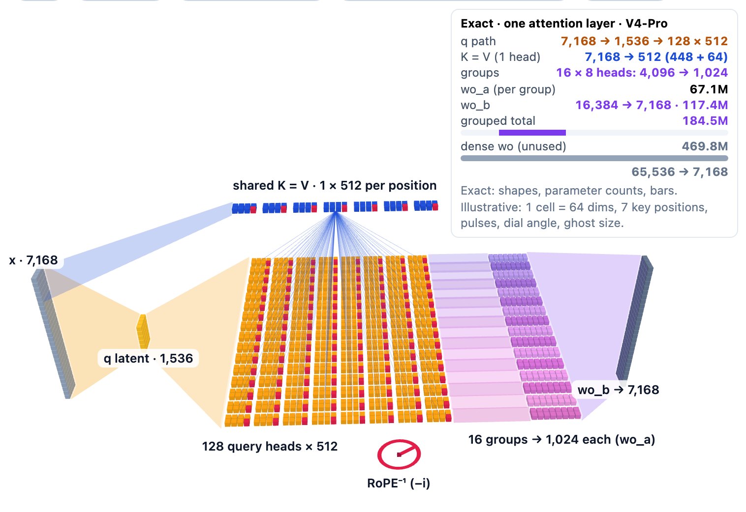
Without one trick, attention would be bigger still. A dense output projection from 128 heads × 512 = 65,536 dimensions down to 7,168 would need 469.8M parameters per layer. V4’s grouped low-rank projection needs 184.5M, saving about 285M per layer, or about 17.4B across Pro’s 61 layers (derived). For Flash it is 67.1M instead of 134.2M per layer. §3.5 shows how the grouping works.

How we counted

• Attention core per layer: wq_a (7,168 × 1,536) + wq_b (1,536 × 65,536) + wkv (7,168 × 512) + wo_a (16 groups × 1,024 × 4,096) + wo_b (16,384 × 7,168) = 11.0M + 100.7M + 3.7M + 67.1M + 117.4M = 299.9M for Pro. Flash: 4.2M + 33.6M + 2.1M + 33.6M + 33.6M = 107.0M.
• Compressors and indexers: a CSA layer adds 31.4M (Pro) or 19.1M (Flash) for its KV compressor, the indexer’s own compressor, the indexer query projection, and its head weights; an HCA layer adds a compressor of 7.41M or 4.26M. Window-only layers add nothing.
• Experts: one SwiGLU expert has three matrices, 3 × 7,168 × 3,072 = 66.1M (Pro) or 3 × 4,096 × 2,048 = 25.2M (Flash). The router is 384 × 7,168 (or 256 × 4,096) per layer.
• Left out: RMSNorm weights, attention sinks, and the mHC mixing weights (24 × 28,672 = 688,128 per sublayer in Pro, about 84M across the model).
• The MTP layer: it would add about 25.7B to Pro (bringing our count to about 1,599B, matching “1.6T”) and about 6.6B to Flash (about 290.6B, above the official 284B). Pro’s count rounds to 1.6T either way, but Flash’s matches 284B only without the MTP layer. So it is unclear whether the official totals include it, and we treat the agreement as approximate.
• Counting the embedding table as “active” follows a common convention; a token only reads one row of it.

3. The Attention Core: One 512-Number Vector per Token, Shared by 128 Heads

Every V4 attention layer, whatever keys it is handed, runs the same core computation. This section answers one question: what happens once a layer has its list of keys? The one idea is radical sharing. Each cached position stores a single vector, and that one vector acts as the key and the value for every query head at once. The rest of the design (wide heads, a small query bottleneck, a position fix on the output, and a cheaper output projection) exists to make that sharing work.

3.1 Idea first: K = V, one head

In a standard multi-head layer, each head has its own key and its own value for every token. V4 keeps exactly one 512-number vector per cached entry. That entry is a raw token in the 128-token window or a compressed block from §4. All query heads (128 in Pro, 64 in Flash) read the same vector, and they use it twice: to score it (as a key) and to average it (as a value).

This is Multi-Query Attention (MQA), where all query heads share one key/value head, pushed one step further: the key and the value are the same vector. The configs set num_key_value_heads to 1 and head_dim to 512, and the reference code builds each raw (window) entry with one projection, wkv = Linear(dim, 512); compressed entries come from the compressor (§4). The technical report names the design “Shared Key-Value MQA”: each entry “serves as both attention key and value.”

In plain terms, take one Pro token in one layer. A classic layer with 128 separate 512-wide keys and values would store $128 \times 512 \times 2 = 131{,}072$ numbers for that token. V4 stores 512, which is 256 times fewer (our arithmetic, for illustration only).

	Per-head keys/values (classic multi-head attention, MHA)	MLA (DeepSeek-V2/V3, GLM-5.3)	V4 shared-KV MQA
What is cached per token or entry	one key and one value per head	512-number latent + 64-number RoPE key	one 512-number vector
How heads get their keys and values	read directly	re-expanded per head (or absorbed into the query)	the cached vector is the key and the value
KV up-projection	none needed	yes	none

If you read the GLM-5.3 post (§3), the contrast with MLA matters. MLA also caches a 512-number vector, but as a latent: each head rebuilds its own keys and values from it through up-projection matrices, and position travels in a separate 64-number key. V4 has no up-projection at all. Its 512 numbers are used as they are, and position lives inside them (§3.3).

Where the numbers come from

• Configs (DeepSeek-V4-Pro and DeepSeek-V4-Flash config.json): head_dim 512, num_key_value_heads 1, num_attention_heads 128 (Pro) and 64 (Flash), qk_rope_head_dim 64. The report’s own hyperparameter lists give the same values ($c = 512$, $n_h$ = 128 / 64).
• Reference code (inference/model.py, class Attention; the file is identical in the Pro and Flash repos): wkv = Linear(dim, head_dim) followed by kv_norm = RMSNorm(512). The attention kernel sparse_attn (kernel.py) takes kv as one [batch, n, 512] tensor with no head axis, and the same tensor feeds both the score product and the weighted sum.
• Naming: the class docstring still says “Multi-head Latent Attention (MLA)”, but the structure is single-head MQA with K = V, and the report calls it “Shared Key-Value MQA” (Eqs. 18-19).
• Storage: the report stores the 64 RoPE dimensions in BF16 and the other 448 in FP8, “nearly half” of pure BF16. By our count that is $448 \times 1 + 64 \times 2 = 576$ bytes per entry instead of 1,024. §4.3 covers what is cached per layer.

One systems consequence follows directly, and it is our reading of the kernel rather than a claim the report makes. In sparse_attn, each block of 64 gathered key rows is loaded into fast on-chip memory once. That single copy serves the score product and, a few lines later, the weighted sum for every head on the GPU (up to 128 in Pro), so one read does up to $2 \times 128$ jobs. That suits decoding, where reading the cache is the bottleneck.

3.2 The query path: low-rank latent shared with the indexer

The key side is a single projection. The query side is wider, because every head needs its own 512-number query. V4 builds those queries through a narrow bottleneck, a latent, the same low-rank trick MLA uses for its queries. Step by step for one Pro token (Flash in parentheses):

1. Down-project. The hidden state $x$ (7,168 numbers; Flash 4,096) goes through wq_a to a 1,536-number latent (Flash 1,024).
2. Normalize the latent. q_norm, an RMSNorm with learned weights, gives the latent $c^Q$, called qr in the code.
3. Up-project. wq_b expands $c^Q$ to $128 \times 512 = 65{,}536$ numbers (Flash $64 \times 512 = 32{,}768$), one 512-number query per head.
4. Rescale each head. Every head’s query is divided by its own root mean square, so each head ends up with RMS 1. This step has no learned weight.
5. Key side. In parallel, wkv maps $x$ to the 512-number window entry, and kv_norm (an RMSNorm with learned weights) normalizes it.

The report writes the same path as two matrices:

\[c^Q_t = h_t\, W^{DQ}, \qquad [\,q_{t,1};\, q_{t,2};\, \dots;\, q_{t,n_h}\,] = c^Q_t\, W^{UQ}\]

In plain terms: squeeze the token to 1,536 numbers, then fan it out to 128 heads. By our count from the shapes, wq_a plus wq_b hold about 111.7M parameters in Pro, against 469.8M for a direct 7,168-to-65,536 projection.

The normalization steps are there for stability. The report says the RMSNorm on each query head and on the single KV head “avoids exploding attention logits,” and that this is why V4 does not use QK-Clip, a logit-capping trick (Liu et al., 2025), with its Muon optimizer (§10). Normalization caps how large a logit can get. Here is a tiny example of that ceiling.

In plain terms: after step 4, a 512-number query with RMS 1 has length $\sqrt{512} \approx 22.6$. If the key also had RMS 1 (that is, the learned kv_norm weights all equal to 1), their dot product could reach at most 512. Times the softmax scale $512^{-1/2}$, the logit can never exceed about 22.6, however large the hidden state grows (our arithmetic; the learned weights move this ceiling but keep it finite).

The latent $c^Q$ has a second user. In CSA layers the lightning indexer, the small scorer that picks which compressed blocks to read, builds its own queries from the same qr with a separate up-projection. The report states that “the latent query vector is shared with that used for the indexer queries.” §5.2 covers the indexer side.

Implementation notes

• Code (model.py, Attention.forward): qr = q = self.q_norm(self.wq_a(x)), then q = self.wq_b(q) unflattened to [heads, 512], then q *= torch.rsqrt(q.square().mean(-1, keepdim=True) + self.eps). The indexer is called as self.indexer(x, qr, ...).
• Paper versus code: the report describes an “RMSNorm operation on each head of the queries.” In the reference code that per-head step carries no learned scale; the learned scales sit in q_norm (on the 1,536-number latent) and kv_norm (on the 512-number entry). Compressed entries pass through the compressor’s own RMSNorm (§4).
• Miles, the training framework, does the same: query down-projection, norm, up-projection, then a per-head RMS rescale in FP32 without a weight.
• Parameter counts (derived from config shapes, no bias terms since attention_bias is false): Pro wq_a $7{,}168 \times 1{,}536 \approx 11.0$M, wq_b $1{,}536 \times 65{,}536 \approx 100.7$M, wkv $7{,}168 \times 512 \approx 3.7$M. Flash: 4.2M, 33.6M, and 2.1M.

3.3 Partial RoPE and the inverse rotation on the output

Attention needs to know where tokens sit. RoPE supplies this by rotating pairs of query and key dimensions through an angle proportional to position, so a query-key score depends only on their distance. V4 rotates only part of each vector. Of the 512 numbers in every query head and every KV entry, the first 448 carry no position (NoPE, “no position embedding”) and the last 64 are rotated.

That layout is a small version of MLA’s decoupled RoPE, with one twist. In MLA, the rotated key is a separate small vector used only for scoring. In V4, the rotated 64 dimensions sit inside the entry that is also the value. So the weighted sum the head returns contains rotated pieces, each tagged with its own key’s absolute position.

The report spells out the problem and the fix. Since KV entries “serve as both attention keys and values, the naive core attention outputs will carry absolute position embeddings.” As a countermeasure, V4 applies “RoPE with position $-i$ on the last 64 dimensions of each” output. The report’s notation is loose here; the reference code makes clear the angle is minus the query’s position: after the attention kernel, it rotates the output’s last 64 dimensions by the conjugate of the query’s rotation.

Why that works, for one rotated pair of numbers. Let $R(\phi)$ rotate a 2-D vector by angle $\phi$, let $\theta$ be the pair’s frequency, and let $u_j$ be entry $j$’s pair before rotation. The head’s output pair is $\sum_j p_j R(\theta j)\, u_j$, where $p_j$ are the attention weights. Rotating it back by the query’s position $i$ gives

\[R(-\theta i) \sum_j p_j\, R(\theta j)\, u_j \;=\; \sum_j p_j\, R\big(\theta (j - i)\big)\, u_j ,\]

because 2-D rotations add their angles.

In plain terms: take $\theta = 10^\circ$, a key at position 3, and a query at position 5. The key’s pair was stored rotated by $30^\circ$; the output is turned back by $50^\circ$, so that key contributes at a net $-20^\circ$. Move both tokens 100 positions later (103 and 105) and the net angle is still $-20^\circ$. What reaches the next layer depends on the distance between query and key, not on where the pair sits in the document.

The report gives the purpose in one line: with the inverse rotation, “the contribution of each KV entry to the core attention outputs will also be related to the distance between the query and the KV entry.” Why DeepSeek preferred this over keeping a separate rotated key, as MLA does, the sources do not say. Our reading is that it lets one 512-number vector do all the work without a second cached piece.

Implementation notes

• Code (model.py): apply_rotary_emb(q[..., -64:], freqs_cis) and the same on kv[..., -64:] before attention; after attention, apply_rotary_emb(o[..., -64:], freqs_cis, True), where True means “use the conjugate”, that is, rotate by minus the angle. freqs_cis is indexed by the query positions, so the inverse turns each output back by its own query’s position. Miles does the same in training, right after its sparse-attention kernel.
• Pairing: the code views the 64 dimensions as 32 complex numbers made from adjacent pairs, so each frequency rotates dimensions $(2k, 2k{+}1)$.
• Precision: the reference code fake-quantizes the 448 NoPE dimensions of each window entry to FP8 (blocks of 64) to match quantization-aware training, while “rope dims stay bf16 for positional precision” (code comment). This matches the report’s mixed BF16/FP8 storage format.
• Positions of compressed entries: a compressed block is rotated as if it sat at its first token’s position (§4.2), so $j$ above is that position.
• Frequencies: compressed layers use RoPE base 160,000 with YaRN; window-only layers (Flash’s layers 0 and 1, and the MTP layer in both models) use base 10,000 without YaRN (§2.2, §9).

3.4 One softmax, a sink, and the window

Each layer hands the core a single list of positions to read. The first part is always the sliding window: the last 128 raw tokens, including the current one. The second part depends on the layer type: top-k compressed blocks in CSA layers (§5), every completed compressed block in HCA layers (§6), and nothing in window-only layers. The code concatenates the two parts into one index list.

One kernel, sparse_attn, then attends over that whole list in a single pass. Raw window entries and compressed entries live in the same 512-number space, so they are scored against the same query and compete in one softmax. There is no separate softmax per part and no learned gate that mixes a “window output” with a “compressed output”. The code has no such branches or weights.

On top of that softmax sits an attention sink: one learned number per head, $z’_h$, that joins the denominator but brings no value with it. The weight of head $h$ for query $i$ on entry $j$ is as follows (Eq. 27; the logit definition and the $1/\sqrt{512}$ scale come from the reference code):

\[s_{h,i,j} \;=\; \frac{\exp(z_{h,i,j})}{\sum_k \exp(z_{h,i,k}) \;+\; \exp(z'_h)}, \qquad z_{h,i,j} = \frac{q_{i,h} \cdot c_j}{\sqrt{512}},\]

where $c_j$ is the shared entry from §3.1. The head’s output is $o_{i,h} = \sum_j s_{h,i,j}\, c_j$.

In plain terms: suppose a head sees three entries with logits 2, 1, and 0, and its sink logit is 1. Without the sink the weights would be 0.665, 0.245, and 0.090, summing to 1. With the sink they become 0.534, 0.197, and 0.072, summing to 0.803. The missing 0.197 goes to “nothing”. The report puts it this way: the sink lets each head make its total attention “not equal to 1, and even to be near 0.” A head with nothing useful to read can stay quiet.

Implementation notes

• Index list (model.py): get_window_topk_idxs gives the 128 window slots (padded with $-1$ early in the sequence); compressed indices come from the indexer (ratio 4) or from get_compress_topk_idxs (ratio 128), and torch.cat joins them. During prefill the code attends over [raw kv of all tokens ; compressed kv]; during decode the window is a 128-slot ring buffer at the front of each layer’s cache.
• Kernel (kernel.py, sparse_attn): gathers 64 rows at a time, masks $-1$ indices to $-\infty$, and keeps a FlashAttention-style running maximum and running sum. After the loop it adds exp(attn_sink[h] - max) to the sum and only then divides. The sink touches the denominator only.
• Scale: softmax_scale = head_dim ** -0.5 $= 512^{-1/2}$.
• attn_sink is an FP32 parameter with one entry per query head (128 in Pro, 64 in Flash). The report cites OpenAI (2025) and Xiao et al. (2024) for the trick.

3.5 Grouped low-rank output projection

Wide heads have a price at the exit. In Pro, the 128 head outputs together hold $128 \times 512 = 65{,}536$ numbers, and they must be mapped back to the 7,168-number hidden state. A single dense output matrix would need $65{,}536 \times 7{,}168 \approx 469.8$M parameters in every layer. The report says this “will impose a substantial computational burden,” and replaces it with a two-stage grouped output projection:

1. Split. The 128 heads form $g = 16$ groups of 8 consecutive heads; each group’s output is $8 \times 512 = 4{,}096$ numbers.
2. Squeeze each group. Each group gets its own matrix (wo_a, one slice per group) that maps its 4,096 numbers to 1,024 (o_lora_rank).
3. Concatenate. The 16 squeezed outputs make $16 \times 1{,}024 = 16{,}384$ numbers.
4. Mix. One dense matrix, wo_b, maps 16,384 numbers to the 7,168-number hidden state.

Flash follows the same recipe at its size: 64 heads in 8 groups of 8 heads (4,096 numbers each), each squeezed to 1,024, giving 8,192 numbers, then mapped to 4,096.

In symbols, with $o^G_{t,k}$ the 4,096 numbers of group $k$:

\[o'_{t,k} = o^G_{t,k}\, W^{A}_k \in \mathbb{R}^{1024}, \qquad \hat{o}_t = [\,o'_{t,1};\, \dots;\, o'_{t,g}\,]\, W^{B} \in \mathbb{R}^{d}\]

In plain terms: group 3 in Pro is heads 24 to 31 (counting from 0). Its slice of wo_a turns their 4,096 numbers into 1,024 and holds $1{,}024 \times 4{,}096 \approx 4.19$M parameters. Sixteen such slices plus wo_b replace the one big matrix.

Per layer (derived from config shapes)	Pro	Flash
Head outputs ($n_h \times 512$)	65,536	32,768
Groups × heads per group	16 × 8	8 × 8
wo_a (all groups)	67.1M	33.6M
wo_b	117.4M	33.6M
Grouped total	184.5M	67.1M
Dense output matrix, for comparison	469.8M	134.2M

V4-Pro splits its 128 attention heads into 16 groups, projects each group from 4,096 to 1,024 with its own matrix (wo_a), then maps the concatenated 16,384 values to 7,168 with one dense wo_b. That is 184.5M parameters per layer instead of 469.8M for a single dense output matrix. Open the full-size SVG.

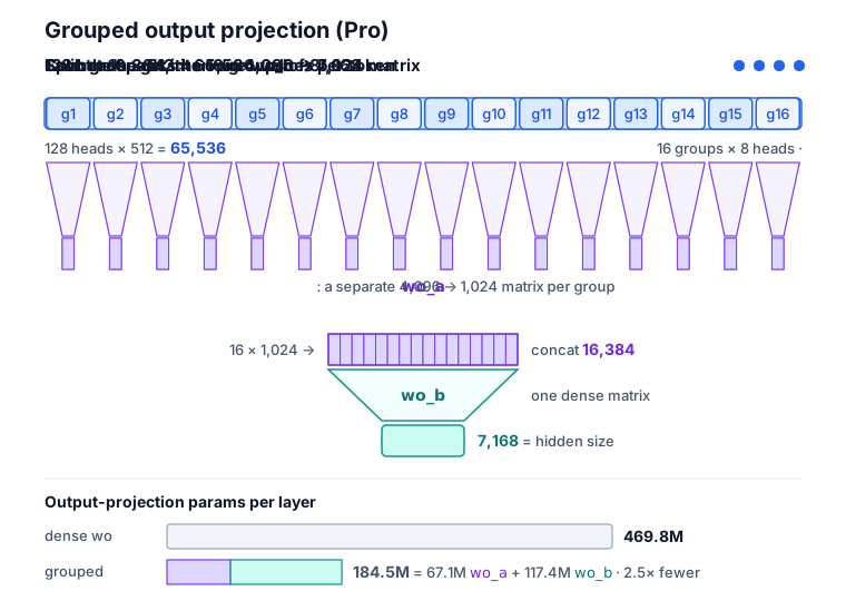
The saving is about 285M parameters per layer in Pro and 67M in Flash, by our count. Compute per token scales the same way, because a matrix-vector product costs about two operations per weight: roughly 369M versus 940M operations per token per Pro layer (derived). This is where the cost of 512-wide heads is paid back.

Our reading of the structure: the first stage is block-diagonal, so each group mixes only its own eight heads. The whole projection is then a sum of 16 pieces, one per group, and each piece passes through 1,024 numbers, so each group’s contribution has rank at most 1,024; the full map can still reach rank 7,168. This per-group low-rank structure is why the code calls it a “grouped low-rank” projection and names the width o_lora_rank. The report does not analyze how much quality this costs.

Implementation notes

• Code (model.py): wo_a = ColumnParallelLinear(n_heads*head_dim // n_groups, n_groups*o_lora_rank) and wo_b = RowParallelLinear(n_groups*o_lora_rank, dim). In the forward pass, o is viewed as [batch, seq, groups, 4096], wo_a.weight as [groups, 1024, 4096], and torch.einsum("bsgd,grd->bsgr", o, wo_a) applies each group’s own slice.
• Precision: the reference code builds wo_a in BF16; a comment notes that wo_a is FP8 in the checkpoint and an FP8 einsum would be faster.
• Parallelism (our reading): the code divides groups across GPUs (n_local_groups = n_groups // world_size), just as it divides heads. Each GPU can apply wo_a to its own heads without communicating, and only the row-parallel wo_b needs a sum across GPUs. Miles uses the same split: a column-parallel per-group projection (linear_o_group_proj) followed by a row-parallel linear_proj, and it asserts o_lora_rank = 1,024.
• Configs: o_groups 16 (Pro) and 8 (Flash), o_lora_rank 1,024 in both; the report’s $g$ and $d_g$ match.

The 3D model below steps through the whole layer for either model, from the query path to the grouped output projection.

One DeepSeek-V4 attention layer, every shape exact: 128 query heads of 512 dims (64 in V4-Flash) all read a single 512-d vector per key position that is both key and value, and only the last 64 dims carry RoPE, rotated back at position −i on the output. Outputs leave through 16 groups (8 in Flash) squeezed to 1,024 each, so the output projection needs 184.5M parameters per layer instead of 469.8M for a dense wo (Flash: 67.1M vs 134.2M).

4. The KV Compressor: Learned Pooling of 4 or 128 Tokens

Every compressed layer in V4 needs a short memory: one stored entry for every few tokens instead of one per token. The compressor builds it. It is a weighted average with a twist: the model learns, separately for each of the 512 channels, which tokens in a block deserve the weight. CSA layers squeeze every 4 tokens into one entry, HCA layers every 128.

4.1 Idea: average, but let the model choose the weights per channel

Mean pooling would give each token in a block the same say. V4’s compressor instead projects every token twice: once into a value $v$ (what the token contributes) and once into a gate score $s$ (how loudly it should speak). Both have one number per channel of the 512-channel entry, so each channel gets its own score (ratio 4 doubles the projection; §4.2). A softmax over the tokens of the block turns the scores into weights, one set per channel, and the entry is the weighted sum of the values.

For a block of $r$ tokens (the compression ratio, 4 or 128), entry $i$ and channel $c$ (written for the plain, non-overlapped case; §4.2 adds the overlap at ratio 4):

\[s_j = W_{\text{gate}}\, x_j + B_{\,j \bmod r}, \qquad v_j = W_{\text{kv}}\, x_j, \qquad C_{i,c} = \sum_{j \in \text{block } i} \frac{\exp(s_{j,c})}{\sum_{j' \in \text{block } i} \exp(s_{j',c})}\; v_{j,c}\]

Here $x_j$ is token $j$’s input to the attention layer (the normalized hidden state, 7,168 numbers in Pro and 4,096 in Flash). $B$ is a small learned table with one row per slot in the block. It lets the gate prefer, say, the last token of every block. The paper writes the same thing as Eqs. 20–23 (HCA) and Eqs. 9–12 (CSA, with the overlap described in §4.2).

In plain terms, here is a toy block of 4 tokens and two channels (made-up numbers):

	token 0	token 1	token 2	token 3	entry
channel A: value $v$	2	4	6	8
channel A: score $s$	0	0	0	$\ln 5$
channel A: weight	0.125	0.125	0.125	0.625	6.5
channel B: value $v$	2	4	6	8
channel B: score $s$	1	1	1	1
channel B: weight	0.25	0.25	0.25	0.25	5.0

Channel B’s equal scores reproduce the plain mean (5.0). Channel A puts most of its weight on token 3 and lands at 6.5. Mean pooling is one point in the space the compressor can learn; it is free to leave it, channel by channel. Our reading: this is attention pooling with a learned per-channel scorer. The reference code’s docstring calls it “learned gated pooling”.

Each compressor is small. It holds two projections ($W_{\text{kv}}$, $W_{\text{gate}}$), the slot-bias table $B$, and an RMSNorm over the 512-dim output:

Compressor (derived from the configs)	Pro, ratio 4 (CSA)	Pro, ratio 128 (HCA)	Flash, ratio 4	Flash, ratio 128
projection width ($W_{\text{kv}}$ and $W_{\text{gate}}$ each)	7,168 → 1,024	7,168 → 512	4,096 → 1,024	4,096 → 512
slot bias $B$	4 × 1,024	128 × 512	4 × 1,024	128 × 512
parameters (by our count)	~14.7M	~7.41M	~8.39M	~4.26M

The ratio-4 projections are twice as wide (1,024) because of the overlap explained next. For scale, one Pro routed expert has about 66.1M parameters (by our count, §8).

Where the numbers come from

• Class Compressor in the official inference/model.py (shipped with both the Pro and Flash repos). Docstring: “Compresses KV cache via learned gated pooling over compress_ratio consecutive tokens.” wkv and wgate are Linear(dim, coff * head_dim), ape is a [compress_ratio, coff * head_dim] parameter (the slot bias $B$; “ape” reads as absolute position embedding, and the V4.1-Flash report calls it “absolute positional embedding”), norm is RMSNorm(head_dim). coff is 2 when the ratio is 4 and 1 otherwise; head_dim is 512.
• The weighted sum is literally (kv * score.softmax(dim=2)).sum(dim=2): the softmax runs along the token axis, independently for every channel. The formula above is our transcription of that line.
• hidden_size 7,168 (Pro) and 4,096 (Flash), head_dim 512 in both configs; ratios 4 and 128 in compress_ratios and in the paper’s model setups.
• Parameter counts are ours: Pro CSA $2 \times 7{,}168 \times 1{,}024 + 4 \times 1{,}024 + 512 = 14{,}684{,}672$; Pro HCA $2 \times 7{,}168 \times 512 + 128 \times 512 + 512 = 7{,}406{,}080$; Flash CSA 8,393,216; Flash HCA 4,260,352. A CSA layer also has a second, narrower compressor inside its indexer (§5.2), not counted here.
• Precision: the checkpoint stores wkv/wgate in BF16, and the reference code upcasts them and the input to FP32 (“compression need fp32”). The compressor weights are not FP8-quantized.

4.2 Ratio 4 (CSA) overlaps; ratio 128 (HCA) does not

A 4-token block is tiny. One way to see it (our reading of the code’s “smoother compression boundaries”): if every token belonged to exactly one entry, a phrase split across a block boundary would land in two unrelated summaries. CSA’s compressor lets each entry also read the block before it, so neighboring entries share 4 tokens. HCA’s 128-token blocks do without.

Here is the ratio-4 path in a Pro CSA layer, with real shapes for a sequence of $n$ tokens:

1. Project twice, 1,024 wide. $v = W_{\text{kv}} x$ and $s = W_{\text{gate}} x$ are both $[n, 1{,}024]$. The slot bias $B$ ($[4, 1{,}024]$) is added to the scores by each token’s slot in its block.
2. Cut into blocks of 4: $[n/4,\ 4,\ 1{,}024]$.
3. Build an 8-slot window per entry, 512 wide. Slots 0–3 hold the previous block’s 4 tokens, using channels 0–511 of their projections. Slots 4–7 hold the current block’s 4 tokens, using channels 512–1,023. Result: $[n/4,\ 8,\ 512]$.
4. Softmax over the 8 slots, separately for each of the 512 channels, then take the weighted sum: $[n/4,\ 512]$.

So entry $i$ pools tokens $4i-4$ through $4i+3$, and consecutive entries start 4 tokens apart. Every token feeds two entries: as “previous” through the first half of the projection and as “current” through the second half. The two halves have separate weights, so a token can say different things to each entry. Entry 0 has no previous block; its first 4 slots get value 0 and score $-\infty$, which means weight 0.

The paper describes the same thing as two series, $C^a$ for the current block and $C^b$ for the previous one, normalized together “across the total of $2m$ elements” (Eqs. 9–12). Flash uses identical widths: only the input side (4,096) differs.

DeepSeek-V4's compressor turns a block of tokens into one 512-d KV entry by a learned, per-channel softmax-weighted sum. At ratio 4 (CSA) each entry also reads the previous block, so entries overlap with stride 4; at ratio 128 (HCA) blocks do not overlap. (Weights are illustrative.) Open the full-size SVG.

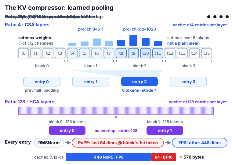
Ratio 128 is the plain version. The projection is 512 wide, there is one series, and each entry pools exactly its own 128 tokens: tokens $128i$ through $128i+127$, stride 128. The paper says HCA “does not perform overlapped compression”. The reference code’s docstring gives the reason for the overlap at ratio 4 (“for smoother compression boundaries”); neither source says why HCA skips it. Our guess (interpretation): with 128 tokens per entry, a boundary cut matters less in relative terms, and doubling the width would double the compressor’s cost.

After pooling, both ratios apply the same three steps to the 512-number entry:

1. RMSNorm over the 512 channels, with learned weights.
2. RoPE on the last 64 dims, at the position of the first token of the entry’s own block: positions 0, $r$, $2r$, and so on. An overlapped ratio-4 entry reaches back to token $4i-4$ but is still rotated as position $4i$.
3. FP8 rounding on the other 448 dims (simulated in the reference code to match quantization-aware training); the 64 RoPE dims stay in BF16. This is the same 448 + 64 split as the window’s raw KV (§3.1).

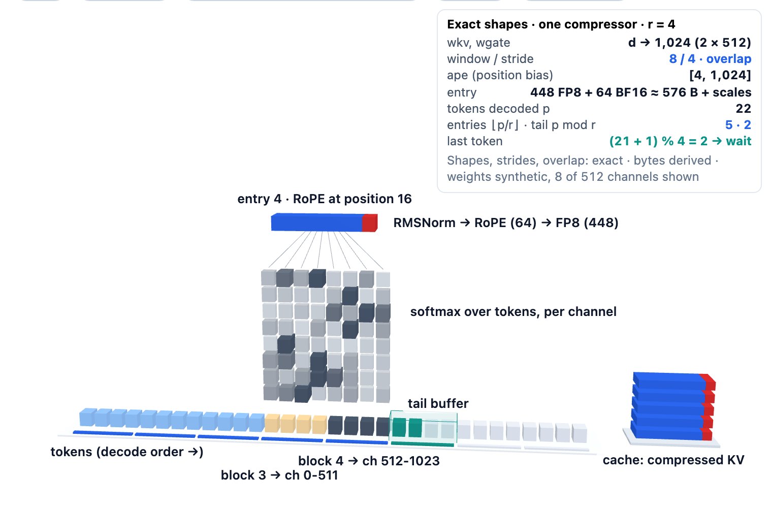
An entry appears only when its block is complete. In decoding, a ratio-$r$ compressor emits a new entry when token position $p$ satisfies $(p+1) \bmod r = 0$. A query at position $t$ can use entry $i$ only if $\lfloor (t+1)/r \rfloor > i$. The tokens of the unfinished block are never compressed early; the 128-token window covers them. For ratio 128 this is just enough: at most 127 tokens can be waiting, and the window holds 128 (derived from the index rules).

In plain terms, take a 10-token prompt (positions 0–9):

• CSA layer (ratio 4). Entry 0 pools tokens 0–3 (position 0). Entry 1 pools tokens 0–7 (tokens 0–3 as “previous”, 4–7 as “current”; position 4). Tokens 8 and 9 wait. The query at position 9 can see entries 0 and 1 plus raw tokens 0–9 in the window.
• HCA layer (ratio 128). No entry exists yet; all 10 tokens wait, and the window alone covers them. Entry 0 will appear when token 127 arrives.

Recent tokens can therefore show up twice: raw in the window and pooled inside a completed entry (always in HCA, which reads every entry; in CSA only when the indexer picks that entry). Both kinds of key go into the same single softmax (§3.4).

The 3D model below lets you toggle between the two ratios, highlight the overlap, and step tokens in one at a time.

DeepSeek-V4's KV compressor turns a window of raw tokens into one cached entry with a per-channel softmax over the tokens (gate score + learned position bias). At ratio 4 (CSA) each entry pools 8 overlapping tokens at stride 4; at ratio 128 (HCA) it pools 128 tokens with no overlap. Then RMSNorm, RoPE on 64 dims (BF16) and FP8 on the other 448.

Implementation notes

• overlap = compress_ratio == 4 and coff = 1 + overlap. The code comment: “When overlap, the first half of dims is for overlapping compression, second half for normal.” overlap_transform builds the [b, s/r, 2r, d] window: new[:, :, r:] = x[:, :, :, d:] (current block, second half) and new[:, 1:, :r] = x[:, :-1, :, :d] (previous block, first half), with fill value 0 for kv and -inf for score.
• The slot bias is added before the overlap transform, so slots 0–3 carry ape[:, :512] and slots 4–7 carry ape[:, 512:]. This matches the paper’s two biases $B^b$ (previous) and $B^a$ (current). The paper’s $W^{aKV}$ and $W^{bKV}$ are the two halves of the code’s single wkv; likewise for $W^{aZ}$, $W^{bZ}$ and wgate.
• RoPE positions: prefill uses freqs_cis[:cutoff:ratio] (positions $0, r, 2r, \dots$); decode uses freqs_cis[start_pos + 1 - ratio], the first position of the block that just finished. Compressed layers use compress_rope_theta 160,000 with YaRN (§9).
• FP8: act_quant(kv[..., :-64], 64, ...) rounds the 448 NoPE dims in blocks of 64 with UE8M0 (power-of-two) scales, in place. The indexer’s own compressor (rotate=True, head dim 128) instead applies a Hadamard rotation and FP4 rounding to the whole vector (§5.2).
• Visibility: HCA lists compressed entries $0 \dots \lfloor (t+1)/128 \rfloor - 1$ (get_compress_topk_idxs); the CSA indexer masks entries with index $\ge \lfloor (t+1)/4 \rfloor$. The paper states the same rule and names its consequence, “a query cannot access information from other tokens within its own compressed block”, as one reason for the window.
• Miles, the open training implementation, uses the same overlap rule and stride-$r$ RoPE positions. Its compressor matmul is BF16 × BF16 with FP32 output, chosen to match SGLang’s rollout kernel, where the reference inference code upcasts to FP32 first (§13).

4.3 What is cached

The compressor turns a growing pile of per-token keys into a much shorter list of entries. What a layer keeps between decoding steps depends on its type:

Kept per sequence	CSA layer (ratio 4)	HCA layer (ratio 128)	Window-only layer (Flash layers 0–1, the MTP layer)
Compressed main KV	$\lfloor n/4 \rfloor$ entries × 512 dims	$\lfloor n/128 \rfloor$ entries × 512 dims	none
Compressed indexer keys	$\lfloor n/4 \rfloor$ × 128 dims, FP4 (§5.2)	none	none
Raw window	last 128 tokens × 512 dims	last 128 tokens × 512 dims	last 128 tokens × 512 dims
Uncompressed tail	fewer than 4 tokens (plus the previous block, for the overlap)	fewer than 128 tokens	none

The compressed entries are the only part that grows with the context, at one entry per 4 or 128 tokens. In the paper’s mixed storage format each main entry takes 576 bytes (448 FP8 + 64 BF16, by our count; §3.1). The window and the tail have a fixed size, so the paper keeps them in a fixed-size, per-request “state cache” and treats them like the state of a state-space model.

In plain terms, after a 1,000-token prompt in Pro:

• a CSA layer holds 250 main entries, 250 indexer keys, the 128-token window, and no pending tokens (1,000 is a multiple of 4), though the state still keeps tokens 996–999 for the next entry’s overlap;
• an HCA layer holds 7 entries (covering tokens 0–895), the window, and a tail of 104 tokens (896–999) waiting for token 1,023.

§9 scales this up to a million tokens and compares it with DeepSeek-V3.2.

Implementation notes

• Reference decode state: each compressor keeps kv_state and score_state buffers of shape [batch, coff·r, coff·512] in FP32 (score initialized to $-\infty$). For ratio 4 that is 8 slots × 1,024: the previous block’s 4 projected tokens (needed for the overlap) plus the current block’s. When a block completes, the code concatenates the first-half channels of slots 0–3 with the second-half channels of slots 4–7, applies the softmax over the 8 slots, writes entry pos // ratio, and shifts the current block into the “previous” slots. For ratio 128 it is 128 slots × 512 and no shift.
• So the reference code’s tail holds projected values and gate scores rather than raw hidden states; the paper describes the tail as “all pending tokens and their associated hidden states”. Either way it is bounded by one block.
• The reference code simulates FP8 on the cached KV (“kv could also use fp8 format, though current implementation uses bf16”); the 576-byte figure assumes the paper’s deployed mixed format and ignores FP8 scale bytes.
• How the paper lays out this cache in blocks (Fig. 6) and how it caches prefixes on disk is covered in §9.4.
• Training must agree with this. Miles drops the trailing seqlen % ratio tokens of each packed segment from compression; its docstring says this “matches inference, where a decode token sitting in an incomplete buffer has no compressed entry either”. The paper’s context-parallel scheme likewise discards trailing tokens fewer than the compression ratio m per packed sequence.
• V4.1-Flash later simplifies this compressor, removing both the overlap and the slot bias (§12.4).

5. CSA: Compressed Sparse Attention

How can one layer pick up a fine detail from anywhere in a million tokens while reading only about a thousand things? CSA first shrinks the memory four-fold with the compressor from §4, then lets a cheap scorer, the lightning indexer, pick the few compressed entries worth reading, and it always adds the most recent tokens on top.

5.1 The idea: DSA, but over compressed blocks

DeepSeek-V3.2 introduced DSA: a small lightning indexer scores every earlier token, and the real attention reads only the top 2,048 of them. The GLM-5.3 post explains DSA and the indexer in detail (§5.1–5.2 there). The V4 report describes CSA as exactly this recipe applied after compression: it “first compresses the KV cache of each $m$ tokens into one entry, and then applies DeepSeek Sparse Attention”, with $m = 4$.

For one query token, a CSA layer runs four steps:

1. Main memory. The compressor (§4) has turned every 4 tokens into one 512-number entry, using overlapping 8-token windows.
2. Index memory. A second, smaller compressor has turned the same 4-token blocks into one 128-number index key each.
3. Selection. The indexer scores every completed block and keeps the top $k$: 1,024 in Pro, 512 in Flash.
4. Attention. The selected entries plus the raw keys of the last 128 tokens go into one softmax per head (with that head’s sink); all heads read the same list (§3.4).

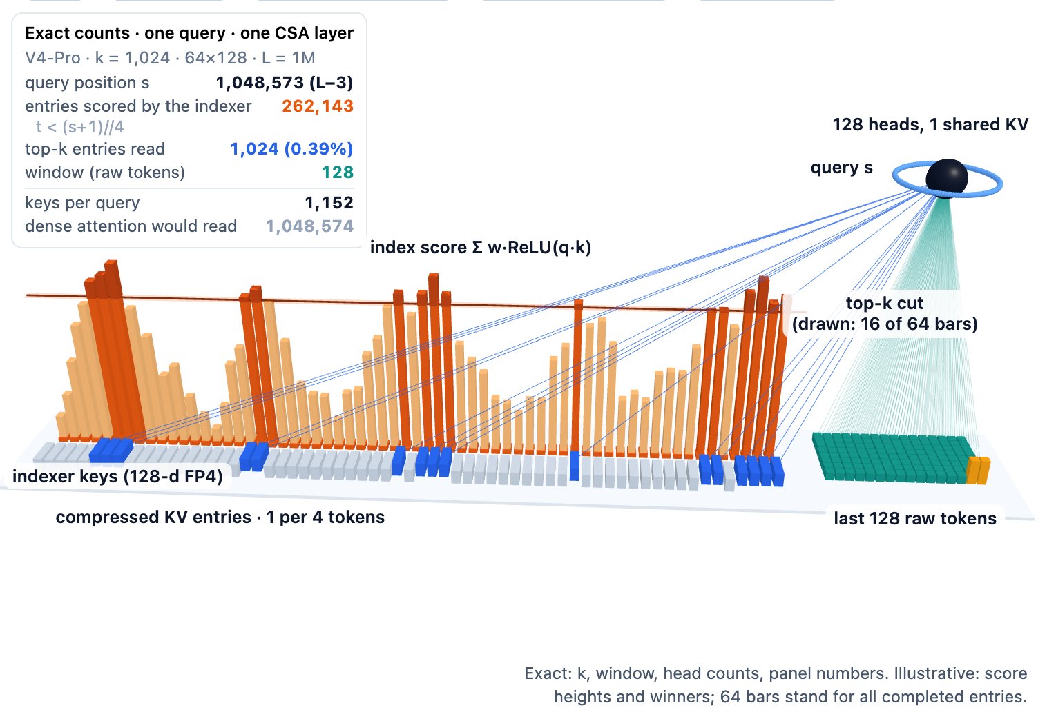
Here is what that means at the full 1M-token context, for a query at the very end:

Per query, per CSA layer	V4-Pro	V4-Flash
Compressed entries in memory ($n/4$)	262,144	262,144
Entries selected (index_topk)	1,024	512
Raw window keys	128	128
Keys in the softmax, at most	1,152	640
Share of compressed entries read	0.39%	0.20%

Rows 1, 4 and 5 are our arithmetic from the config.

In plain terms: the indexer still scans the whole compressed memory, but the expensive part, 128 (Pro) or 64 (Flash) heads attending with 512-wide keys, touches at most 1,152 or 640 keys. That number stays the same at 64K and at 1M. What grows with length is the indexer’s scan over $n/4$ small keys. CSA makes that scan four times shorter than scoring every token, and §5.2 shows how it also makes each step of the scan cheaper.

Where the numbers come from

• $m = 4$, indexer 64 heads × 128 dimensions, top-k 1,024 (Pro) / 512 (Flash), window 128: report §4.2.1 and the configs (compress_ratios, index_n_heads, index_head_dim, index_topk, sliding_window). Config and report agree.
• 1,048,576 / 4 = 262,144 entries; 128 + 1,024 = 1,152 and 128 + 512 = 640 keys; 1,024 / 262,144 ≈ 0.39% and 512 / 262,144 ≈ 0.20%. All are our arithmetic.
• V3.2’s top-2,048 comes from the V3.2 config, as discussed in the GLM-5.3 post. The V4 report only says that V4 uses “a smaller attention top-k” than V3.2, which helps “on short- and medium-length texts”.

5.2 What is different from V3.2’s indexer

The scoring rule is the familiar DSA rule. What changed is what gets scored and how cheaply. The table puts the two side by side. The V3.2 column follows the GLM-5.3 post, whose §5 describes the V3.2 design.

	DeepSeek-V3.2 (DSA)	DeepSeek-V4 (CSA)
One index key per	token	block of 4 tokens (overlapping 8-token window)
Where the keys come from	a projection of each token	their own compressor (ratio 4, 128-wide)
What attention reads after selection	the selected tokens’ cached entries	the selected compressed entries (512-d, key = value)
Top-k	2,048 tokens	1,024 entries (Pro), 512 (Flash)
Plus, every query	nothing extra: no window, and the query’s own token is not forced in (GLM-5.3 post §5.3)	the raw keys of the last 128 tokens (window)

Let us follow one query through the V4-Pro indexer, with shapes from the config and the reference code (Flash in brackets).

1. Index keys, written once per block. The indexer owns a compressor of its own, the same learned pooling as §4 with ratio 4 and overlap, but 128 wide. Each token’s hidden state (7,168 [4,096]) is projected to 2 × 128 numbers for values and 2 × 128 for gate scores. Every completed 4-token block yields one 128-d key. It is RMS-normalized, gets RoPE on its last 64 dimensions, then a Hadamard rotation (a fixed orthogonal mix of the 128 dimensions, see below), then FP4 rounding. The cache holds $n/4$ of these keys.
2. Index queries, reusing the attention’s latent. The main attention already squeezes the token into a 1,536-wide [1,024] query latent (§3.2). The indexer projects that same latent with its own wq_b to 64 heads × 128 = 8,192 numbers, applies RoPE to the last 64 dimensions of each head, rotates, and rounds to FP4. The paper states this sharing explicitly: the latent “is shared with that used for the indexer queries”.
3. Head weights. A small projection weights_proj maps the hidden state to 64 scalars, one per indexer head, scaled by $128^{-1/2}\cdot 64^{-1/2}$.
4. Score every visible block with the formula below, for query position $s$ and block $t$.
5. Keep the best. The selector keeps $\min(k,\ \text{number of visible blocks})$ entries.

\[I_{s,t} \;=\; \sum_{h=1}^{64} w_{s,h}\;\mathrm{ReLU}\!\left(\mathbf{q}_{s,h}\cdot \mathbf{k}_t\right), \qquad \text{block } t \text{ visible iff } t < \left\lfloor \tfrac{s+1}{4} \right\rfloor\]

In plain terms: this is V3.2’s scorer pointed at a catalog four times shorter. Each card in the catalog now stands for a 4-token block, and V4 stores and multiplies the cards in 4-bit floats. The visibility rule means a block becomes selectable only once its last token has arrived. The query’s own unfinished block is left to the window (§5.3).

One query in a DeepSeek-V4 CSA layer: 64 indexer heads score every compressed entry (one per 4 tokens), a top-k cut keeps 1,024 (V4-Pro) or 512 (V4-Flash), and the last 128 raw tokens are added. All heads then share one softmax over at most 1,152 or 640 keys instead of ~1M; the panel gives exact counts, while the bar heights and winners are illustrative.

Two details are easy to miss. The Hadamard rotation is applied to both queries and keys, and an orthogonal rotation leaves every dot product unchanged. In exact arithmetic it does nothing to the scores. The code’s docstring gives the reason: it “spread[s] information across dims before FP8 quant” (the indexer path actually rounds to FP4). In other words, it smears a few large outlier channels across all 128 dimensions so the rounding hurts less. The paper does not discuss it.

Second, the precision trick is a post-training addition. The report’s FP4 quantization-aware training (QAT) caches, loads and multiplies the indexer’s QK activations “entirely in FP4”, and quantizes the index scores from FP32 to BF16. It reports “a 2× speedup for the top-k selector, while preserving a 99.7% recall rate of KV entries”.

The GLM-5.3-Flash “kpool” indexer (§8.5 there) also pools keys over blocks of four. It differs in what happens after selection: GLM expands each chosen block back into its 4 raw tokens, whereas V4 attends to the compressed entries themselves. V4 does not fetch the raw tokens of a selected block; raw tokens enter only through the window.

Implementation notes

• Where it lives. class Indexer in the reference inference/model.py is built only when a layer’s compress ratio is 4. Ratio-128 layers have indexer = None. Its parts are wq_b (1,536 → 8,192 in Pro, 1,024 → 8,192 in Flash), weights_proj (hidden → 64, BF16), and Compressor(ratio 4, head_dim 128, rotate=True) with its own cache of shape [batch, max_seq_len / 4, 128].
• Scale. weights = weights_proj(x) * (128 ** -0.5 * 64 ** -0.5), the indexer head dimension and head count. The ReLU’d dot products are multiplied by these weights and summed over heads.
• FP4 in the code. Queries and compressed keys both go through fp4_act_quant with block size 32 after the Hadamard rotation (rotate_activation). A code comment notes that the stored keys “could also use fp8 format, though current implementation uses bf16”. The reference code simulates the QAT rounding rather than storing packed FP4.
• Parameters (derived). Per CSA layer the indexer adds about 16.7M parameters in Pro (compressor 3.7M, wq_b 12.6M, weights_proj 0.46M) and 10.8M in Flash. Together with the 512-wide main compressor, a CSA layer carries about 31.4M (Pro) / 19.1M (Flash) parameters that an HCA layer lacks or has in smaller form (HCA’s ratio-128 compressor: 7.4M / 4.3M).
• Index convention. The report writes the visibility rule as $s < \lfloor t/m \rfloor$, with $t$ the query. The code, with 0-based positions, uses block < (pos + 1) // 4. A block thus becomes visible at its own last token, the query included. Our reading is that both say the same thing under different indexing.
• Training code differs. Miles applies FP8 QAT with block 128 to the indexer compressor’s output. The reference inference code uses FP4 with block 32. This is a real train/inference precision difference in the open training stack (§13).

5.3 Selection and the window in one softmax

The indexer returns positions in the compressed memory. The attention kernel, however, takes one flat list of row numbers into one buffer. The reference code therefore lays out a single buffer with the raw-token keys first and the compressed entries after them. It shifts every selected entry id by an offset:

• Prefill (whole prompt at once): buffer = [all $L$ raw-token keys of the prompt ; its $\lfloor L/4 \rfloor$ compressed entries], offset = $L$.
• Decode (one token at a time): buffer = [128-slot ring of recent keys ; compressed entries], offset = 128.

The final index list for a query is the 128 window positions followed by the $k$ shifted entry ids. sparse_attn gathers those rows and runs one online softmax (computed in one streaming pass) over all of them, plus the per-head sink (§3.4). There is no second softmax and no gate weighing “local” against “compressed”.

A tiny example. Shrink everything: ratio 4, window 8, $k = 3$, and a query at position 21.

1. Visible blocks: $\lfloor 22/4 \rfloor = 5$, so blocks 0–4 (tokens 0–19). Tokens 20–21 sit in block 5, which is still incomplete.
2. Made-up index scores for blocks 0–4: 0.1, 0.9, 0.0, 0.4, 0.7. The top 3 are blocks 1, 4 and 3.
3. Window: tokens 14–21, which include the query itself.
4. Index list: 8 raw keys + 3 compressed entries = 11 keys, one softmax.

Block 4 covers tokens 16–19 (plus 12–15 through the overlap channels), and those tokens are also in the window. The model sees them twice, once raw and once pooled. Nothing in the code removes such duplicates.

At real size the same arithmetic gives the numbers in §5.1. Take a V4-Pro query at position 9,999: 2,500 blocks are visible, the indexer keeps 1,024 of them, and the window adds tokens 9,872–9,999. That is 1,152 keys. Flash keeps 512 of the 2,500, for 640 keys.

Sparsity only starts once there are more visible blocks than $k$. Pro reaches that at position 4,099 (1,025 visible blocks) and Flash at position 2,051 (513). Before that, the top-k keeps every block, so a CSA layer attends densely over its compressed memory. These thresholds are derived from the code’s $\min(k, \cdot)$.

How the indexer is trained. The report gives the schedule but not the loss. Training starts with “dense attention for the first 1T tokens” in Flash, and Pro “starts with a longer stage of dense attention”. Sparse attention is switched on at the 64K sequence-length stage. First comes “a short stage to warm up the lightning indexer in CSA”, then sparse training for the rest of the run.

The report does not say whether “dense” here means all compressed entries or something else. It does not describe the indexer’s training objective either. V3.2 trained its indexer to match the dense attention distribution (see the GLM-5.3 post, §5.4). Whether V4 does the same, the sources do not say.

Implementation notes

• Index layout. In Attention.forward: offset = kv.size(1) if start_pos == 0 else win. Indexer ids get + offset, and the window ids come first in torch.cat([window_idxs, compress_idxs]). The decode cache is allocated as window_size + max_seq_len // ratio rows.
• Masking. During prefill, entries for blocks that are not yet complete are set to -1, and the kernel masks -1 to $-\infty$. The window list is padded the same way for the first 127 positions.
• Miles builds the same list: window ids, then compressed ids shifted by kv_compress_offset. For packed sequences (THD) it also restricts each query’s top-k to its own segment. A recent Miles commit balances the CSA indexer across context-parallel ranks (§13).
• Report, Figure 3 shows the same pipeline: token-level compressor → compressed KV; a separate compressor → compressed indexer keys; lightning indexer → top-k selector; then concatenation with the sliding-window KV before shared-KV MQA.

6. HCA: Heavily Compressed Attention

CSA keeps detail and pays for it with a selection step, while HCA makes the opposite trade. It compresses so hard that reading everything becomes cheap, so it needs no indexer at all. Every 128 tokens become one entry, and every query reads all of them plus the recent window.

6.1 The idea: compress so hard that dense attention is cheap

The report describes HCA as compressing the KV cache “in a heavier manner, but does not employ sparse attention”. In a ratio-128 layer, step by step:

1. Compress. The compressor from §4 runs with ratio 128 and no overlap. Its projection is a single 512-wide series, with a learned position bias for each of the 128 slots in a block. Every completed block of 128 tokens becomes one 512-d entry. RoPE is applied at the position of the block’s first token.
2. Skip selection. There is no indexer, no index keys and no top-k. The index list is simply all completed entries.
3. Attend. As in CSA, the list is the 128 window positions followed by those entries. One softmax with the per-head sink runs over it. The core is the same shared-key-value MQA with the grouped output projection (§3); the report says so explicitly.

The number of keys per query now grows with the context, but slowly. The table counts keys per query in one layer, with CSA for comparison:

Context	HCA: $128 + \lfloor n/128 \rfloor$	CSA, Pro	CSA, Flash
8K	64 + 128 = 192	1,152	640
64K	512 + 128 = 640	1,152	640
128K	1,024 + 128 = 1,152	1,152	640
1M	8,192 + 128 = 8,320	1,152	640

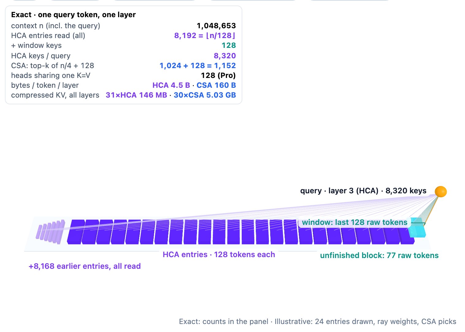
All counts are derived from the config and code, for a query at the end of the context.

In plain terms: up to 128K tokens an HCA layer reads no more keys than a Pro CSA layer, and it never has to scan an index. At 1M it reads 8,320 keys, about 7.2 times as many as CSA’s 1,152. In exchange, each of those keys summarizes 128 tokens, and none of the context is skipped.

The cache is tiny. One entry stores 576 bytes (448 FP8 + 64 BF16 dimensions, §3.1) for 128 tokens, which is 4.5 bytes per token per layer (derived). A CSA layer stores (576 + 64) / 4 = 160 bytes per token, counting its FP4 index key (derived). At 1M tokens one HCA layer holds about 4.7 MB of compressed entries, against about 168 MB for one CSA layer (derived).

A tiny example. Take a query at position 1,000 in an HCA layer.

1. Completed blocks: $\lfloor 1{,}001/128 \rfloor = 7$, so entries 0–6. Together they cover tokens 0–895, and entry 6 carries RoPE position 768.
2. Tokens 896–1,000 (105 tokens, the query included) sit in block 7, which is not finished.
3. The window covers tokens 873–1,000, so all 105 unfinished tokens are present as raw keys. Tokens 873–895 appear twice, raw and inside entry 6.
4. Total: 7 + 128 = 135 keys in one softmax.

This is why the window is not optional. A query can never see its own unfinished block in compressed form. For ratio 128 that gap is 0 to 127 tokens. A 128-token window, which includes the query, is just large enough to cover it in every case.

Where the numbers come from

• Code. HCA layers build a Compressor with ratio 128 (overlap = False, so coff = 1, wkv/wgate 7,168 → 512 in Pro, ape of shape [128, 512]) and set indexer = None. The compressed index list comes from get_compress_topk_idxs, which returns every entry id below (pos + 1) // 128 (shifted by the same offset as in §5.3).
• Report. Eqs. 20–23 define HCA’s single-series compression with a softmax over each block of $m’$ tokens plus a learned positional bias $B \in \mathbb{R}^{m’ \times c}$. §4.2.1 sets $m’ = 128$ for both models.
• Parameters (derived). The HCA compressor has about 7.4M parameters per layer in Pro and 4.3M in Flash, against about 31.4M / 19.1M for CSA’s two compressors plus indexer.
• Bytes (derived). 576 / 128 = 4.5 B; (576 + 64) / 4 = 160 B, where 64 B is a 128-d FP4 index key with its small scale factors ignored. 8,192 × 576 B ≈ 4.7 MB and 262,144 × 640 B ≈ 168 MB per layer at 1,048,576 tokens. Whole-model totals are in §9.

6.2 Why interleave CSA and HCA

The two layer types answer different questions about the past:

	CSA	HCA
Resolution of one entry	4 tokens (8 with overlap)	128 tokens
How much of the past is read	top 1,024 (Pro) / 512 (Flash) entries	every completed entry
Who decides	the lightning indexer	nobody, all are read
Recent tokens	128-token raw window	128-token raw window
Cache per token per layer (derived)	160 B	4.5 B

Fine but selective, or coarse but complete. Think of a long book: a CSA layer re-reads a thousand chosen paragraphs closely, while an HCA layer skims a one-line summary of every page. Both keep the last page in view.

V4 alternates them. From layer 2 on, even layers are CSA and odd layers are HCA. That gives Pro 30 CSA and 31 HCA layers (its first two layers are also HCA) and Flash 21 CSA and 20 HCA (§2.2). The report gives no rationale beyond calling it an “interleaved hybrid configuration” that cuts long-context cost.

Our reading is that alternation lets every few layers of depth see both views: a coarse map of the whole context, and sharp copies of the parts the indexer judges relevant. What one layer finds can then guide what the next one attends to.

One HCA layer: every 128 tokens are pooled into one entry, and the query reads every completed entry plus the 128 newest raw tokens, with no indexer and no top-k. Switch context and model to see the exact key counts, or compare with a CSA layer that keeps only its top-k entries at 4-token resolution.

The animation below puts the two side by side at 1M tokens.

At a 1M-token context, a CSA layer keeps 262,144 fine entries but each query attends only the indexer's top 1,024 plus the 128-token window, while an HCA layer keeps just 8,192 coarse entries and reads every one. Byte costs are derived from the released configs and code (Pro numbers; Flash uses top-512). Open the full-size SVG.

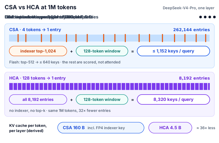
Neither layer type is “the cheap one” at every length. The table in §6.1 shows HCA reading no more keys than Pro’s CSA up to 128K, and more at 1M. CSA, on the other hand, always pays for its indexer scan over $n/4$ keys. The hybrid keeps each kind of layer in the range where its cost is bounded: CSA’s attention by $k$, HCA’s cache by the 128:1 ratio.

Rough per-query work at 1M, one Pro layer (derived)

A rough multiply-add count for the attention-side work of one query, ignoring projections, softmax and precision differences. It is not the report’s FLOPs accounting, which uses “equivalent FP8 FLOPs” for the whole model.

• CSA main attention: 1,152 keys × 128 heads × (512 for scores + 512 for values) ≈ 151M.
• CSA indexer scan: 262,144 keys × 64 heads × 128 ≈ 2.1B, done in FP4 after post-training QAT.
• HCA attention: 8,320 keys × 128 heads × 1,024 ≈ 1.1B.

At this length the indexer scan, not CSA’s sparse attention, is the largest term. Our reading: this fits the report’s emphasis on making exactly this path FP4. Paper-level FLOPs comparisons with V3.2 are in §9.3.

The sources say little about why the ratios are 4 and 128, or why the pattern alternates one-to-one. We found no ablation of either choice in the report. Both remain open questions (§14).

7. mHC: Four Residual Streams, Mixed by a Doubly Stochastic Matrix

A normal transformer has one residual stream: each sublayer reads it and adds its output back. DeepSeek-V4 keeps four copies of that stream side by side and learns, per token, how to blend them before each sublayer, how to write the result back, and how to shuffle signal between the copies. A mathematical constraint on the shuffle keeps 61 layers of this (43 in Flash) from blowing up.

7.1 What V4 inherits and what it adds

The GLM-5.3 post (§8.6) introduced mHC with GLM-5.3-Flash. That post had to take the math from the mHC paper, because we had not inspected the Megatron module that implements it. For V4 we have more: the report writes out the equations, and DeepSeek’s reference code (inference/model.py plus a TileLang kernel in kernel.py) shows every step. This section follows the code.

The report lists mHC as one of V4’s three key upgrades over DeepSeek-V3, next to hybrid attention and the Muon optimizer. Its stated goal is to “strengthen conventional residual connections.” Earlier hyper-connections (HC, Zhu et al., 2025) widened the residual but, in DeepSeek’s words, training “will frequently exhibit numerical instability when stacking multiple layers.” mHC keeps the width and adds a constraint aimed at that instability.

The report’s update rule for one sublayer $F_l$ (attention or MoE) is

\[X_{l+1} = B_l\,X_l + C_l\,F_l\!\left(A_l\,X_l\right), \qquad X_l \in \mathbb{R}^{n_{hc}\times d}\]

with $n_{hc} = 4$ streams of width $d$ (7,168 in Pro, 4,096 in Flash). $A_l$ ($1\times4$) blends the four streams into one sublayer input, $C_l$ ($4\times1$) spreads the sublayer output back over the streams, and $B_l$ ($4\times4$) mixes the streams with each other.

In plain terms: with an ordinary residual, $n_{hc} = 1$ and $A = B = C = 1$, which gives back $x + F(x)$. mHC replaces those three 1s with small learned matrices that change from token to token.

Where the numbers come from

• hc_mult 4, hc_sinkhorn_iters 20, hc_eps 1e-6 in both the Pro and Flash configs; the report’s model setups restate $n_{hc} = 4$ and $t_{\max} = 20$ for both models.
• Report §2.2 (“Manifold-Constrained Hyper-Connections”) gives Eqs. 1–8 used in this section; the three-upgrades list is in the introduction and §2.
• The mHC method itself is from Xie et al. (2026), which the V4 report cites.

7.2 One mixing site, step by step

Every V4 layer has two mixing sites, one around attention and one around the MoE. The residual state for one token is a $4 \times 7{,}168$ block in Pro (28,672 numbers) and $4 \times 4{,}096$ in Flash (16,384). The embedding enters it by being copied four times. At each site the code does five things:

1. Read the whole state. Flatten the four streams into one vector of length $4d$ (28,672 in Pro).
2. Make 24 numbers. Multiply by a learned matrix hc_fn of shape $24 \times 4d$, then divide by the vector’s root mean square. The 24 outputs split into 4 for $A$, 4 for $C$, and 16 for $B$.
3. Shape them. $A$ becomes sigmoid(...), a value in (0, 1) per stream. $C$ becomes 2 * sigmoid(...), in (0, 2). $B$’s 16 raw values go through Sinkhorn normalization (§7.3).
4. Run the sublayer. The input is $\sum_j A_j X_j$, a weighted sum of the four streams (one $d$-wide vector), followed by the usual RMSNorm and then attention or the MoE.
5. Write back. New stream $k$ = $C_k \cdot F(\text{input}) + \sum_j B_{kj} X_j$.

Each of the 24 numbers follows the report’s split of a dynamic and a static part. With $\hat{X}_l = \mathrm{RMSNorm}(\mathrm{vec}(X_l))$, a learned scalar gate $\alpha$ and a learned static bias $S$:

\[\tilde{A}_l = \alpha^{\text{pre}}_l\,\hat{X}_l W^{\text{pre}}_l + S^{\text{pre}}_l,\qquad A_l = \sigma(\tilde{A}_l),\qquad C_l = 2\,\sigma(\tilde{C}_l)\]

and the same form for $\tilde{B}_l$ and $\tilde{C}_l$. The gates $\alpha$ are “initialized to small values,” so (our reading) training starts with the static biases doing most of the work.

In plain terms, take one channel of one token in Pro, with the four streams holding $X = [1.0,\ 0.0,\ 2.0,\ 1.0]$ (illustrative values):

• Blend. With $A = [0.5, 0.5, 0.5, 0.5]$ the sublayer input is $0.5 + 0 + 1.0 + 0.5 = 2.0$. Suppose the sublayer returns $0.4$.
• Mix. Let $B$ have 0.7 on the diagonal and 0.1 elsewhere. New stream $k$ gets $0.7X_k + 0.1 \times$ (the other three), which gives $[1.0,\ 0.4,\ 1.6,\ 1.0]$. The total is still 4.0: mixing only moves signal between streams.
• Add. With $C = [1.2, 0.8, 1.0, 1.0]$ the streams receive $[0.48, 0.32, 0.40, 0.40]$ and become $[1.48,\ 0.72,\ 2.00,\ 1.40]$.

One detail is easy to miss. The four $A$ weights are separate sigmoids, so they need not sum to 1; their sum can be anywhere between 0 and 4. Our reading is that this is harmless because the sublayer’s RMSNorm removes the overall scale right after the blend, so $A$ effectively sets the proportions of the four streams. The report’s own reason for sigmoids on $A$ and $C$ is to keep them “non-negative and bounded … to avoid the risk of signal cancellation.”

Implementation notes: the code behind each step

• Parameters per site (Block.__init__, all float32): hc_attn_fn / hc_ffn_fn of shape $[24,\ 4d]$, where $24 = (2 + 4) \times 4$; hc_*_base $[24]$, which is the report’s static biases $S$; hc_*_scale $[3]$, which holds the three gates $\alpha^{\text{pre}}, \alpha^{\text{post}}, \alpha^{\text{res}}$.
• The RMSNorm is folded in. hc_pre computes mixes = linear(x, hc_fn) * rsqrt(mean(x**2) + eps) on the flattened float32 state. Scaling after the matmul equals normalizing before it, and there is no learned norm weight here (the report’s $\mathrm{RMSNorm}(\mathrm{vec}(X_l))$).
• The split (hc_split_sinkhorn kernel): pre[j] = sigmoid(mixes[j] * scale[0] + base[j]) + eps for $j < 4$; post[j] = 2 * sigmoid(mixes[4 + j] * scale[1] + base[4 + j]); comb[j, k] = mixes[8 + 4j + k] * scale[2] + base[8 + 4j + k] before Sinkhorn. eps is hc_eps = 1e-6.
• Order inside a layer (Block.forward): hc_pre → attn_norm → attention → hc_post, then hc_pre → ffn_norm → MoE → hc_post, each site with its own parameters.
• Index convention. hc_post computes new stream $k$ as $C_k F + \sum_j \texttt{comb}[j,k]\,X_j$, so the code’s comb is the report’s $B_l$ transposed. §7.3 shows why the two descriptions still agree.
• Precision. The coefficient math and the blend run in float32; hc_pre casts its output back to its input’s dtype, and hc_post to the dtype of the sublayer (attention or MoE) output.

7.3 Sinkhorn: forcing the 4 × 4 mixer to be doubly stochastic

The constraint that gives mHC its name sits on $B_l$. It must be doubly stochastic: every entry is non-negative, and every row and every column sums to 1. The report states the two properties that matter:

• Such a matrix has spectral norm at most 1, so the residual mixing is “non-expansive”: it cannot amplify the signal. The report credits this with better numerical stability “during both the forward pass and backpropagation.”
• The set is “closed under multiplication”: the product of all 122 mixers in Pro’s 61 layers (86 in Flash) is again doubly stochastic, so the whole stack stays bounded too.

Unconstrained HC has neither guarantee. A mixer with spectral norm slightly above 1 can grow the signal a little at every site, and over 122 sites a little compounds.

To land on that set, V4 uses the Sinkhorn–Knopp algorithm. Start from the 16 raw numbers, make them positive with $\exp(\cdot)$, then alternate:

\[M^{(0)} = \exp\!\big(\tilde{B}_l\big),\qquad M^{(t)} = \mathcal{T}_r\!\big(\mathcal{T}_c(M^{(t-1)})\big),\qquad B_l = M^{(t_{\max})},\quad t_{\max} = 20\]

where $\mathcal{T}_c$ divides each column by its sum and $\mathcal{T}_r$ does the same for rows. Each step fixes one set of sums and slightly disturbs the other; after a few rounds both are close to 1. The report calls 20 “a practical value.”

In plain terms, on a $2\times 2$ example: start from the rows $(2, 1)$ and $(1, 1)$. Normalizing columns gives the rows $(0.667, 0.5)$ and $(0.333, 0.5)$, which sum to 1.167 and 0.833. Normalizing rows gives $(0.571, 0.429)$ and $(0.4, 0.6)$; now the columns sum to 0.971 and 1.029. One round has cut the worst error from 0.167 to 0.029, and later rounds keep shrinking it.

Because the last step of each round is an exact normalization, the final $B_l$ is exact in one direction and approximate in the other. In the report’s order (columns, then rows) the rows of $B_l$ sum to 1 exactly (up to the tiny 1e-6 eps added to each sum). That direction is the one that matters for the update rule: each new stream is then a weighted average of the old ones.

Four residual streams run through the attention and MoE sublayers of DeepSeek-V4's layer indices 1-3 (counted from 0; types exact from the config). At every sublayer, sigmoid pre weights and 2σ post gains connect the streams to the sublayer, and a 4×4 mixer is pushed to doubly stochastic by 20 Sinkhorn rounds, so stacked mixers stay at about 1× while unconstrained ones grow (matrix values and the 30-layer log-height strip are illustrative).

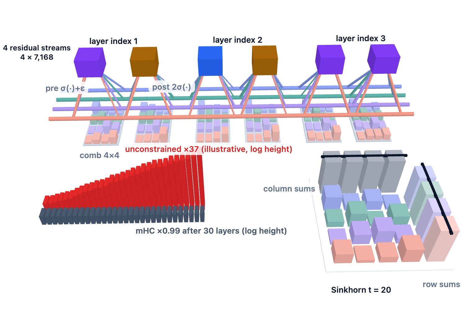
The 3D model above lets you scrub through the 20 Sinkhorn rounds and compare a constrained mixer with an unconstrained one; its matrix values are illustrative.

Implementation notes: Sinkhorn in the kernel, and why the code and the report agree

• The TileLang kernel hc_split_sinkhorn runs one GPU thread block per token and keeps the $4 \times 4$ matrix in on-chip memory.
• Its first round is a row softmax plus eps (which is $\exp$ followed by row normalization), then a column normalization. It then runs sinkhorn_iters - 1 = 19 more rounds of row-then-column normalization, so 20 rounds in total. The later divisions add eps (1e-6) to each sum.
• The code normalizes rows first and columns last, the opposite of the report’s Eq. 8. Its comb is the transpose of the report’s $B_l$ (§7.2 notes), and transposing swaps rows and columns, so the two describe the same computation. In both, every new stream receives weights that sum to 1 exactly, and every old stream hands out weights that sum to approximately 1.
• After a finite 20 rounds the matrix is doubly stochastic only approximately; the guarantees above hold up to that small error.

7.4 What four streams cost

In parameters, almost nothing. Each site’s hc_fn is $24 \times 28{,}672 = 688{,}128$ weights in Pro and $24 \times 16{,}384 = 393{,}216$ in Flash. Over 122 sites (Pro) and 86 sites (Flash), that is about 84.0M and 33.8M weights by our count, roughly 0.005% and 0.01% of the totals. The compute is small as well: at each site, computing the 24 coefficients costs about 1% of one Pro expert’s multiply-adds per token (derived).

The real price is width. Between layers, every token now carries $4d$ numbers instead of $d$: 28,672 instead of 7,168 in Pro. The report says mHC “increases both activation memory consumption and communication volume between pipeline stages,” and lists three countermeasures:

• Fused kernels for mHC in both training and inference.
• Selective recomputation. Most hidden states between layers and all normalized layer inputs are recomputed in the backward pass instead of stored; compute-heavy operations are not recomputed.
• A retuned pipeline schedule. DeepSeek adjusted the overlap in its DualPipe 1F1B (one-forward-one-backward) pipeline schedule to absorb the extra pipeline traffic and run parts of mHC concurrently.

With these, the report puts mHC’s wall-time overhead at “only 6.7% of the overlapped 1F1B pipeline stage.”

At the top of the network the four streams must become one vector again for the LM head. V4 does this with one more learned blend (hc_head): four sigmoid weights computed from the state, the same way $A$ is computed at a mixing site, with no Sinkhorn step and no write-back. The final RMSNorm and the LM head follow. (GLM-5.3-Flash, by contrast, simply averages its four lanes.)

Implementation notes: head, MTP, optimizer, determinism

• hc_head (ParallelHead): hc_head_fn $[4,\ 4d]$, hc_head_base $[4]$, hc_head_scale $[1]$; weights sigmoid(mixes * scale + base) + eps after the same folded RMS normalization. Only the last position’s logits are computed at inference.
• MTP. MTPBlock subclasses Block, so the multi-token-prediction layer carries its own two mixing sites and its own hc_head (hc_head_fn / _base / _scale). The 122 / 86 counts above cover main layers only.
• Optimizer. V4 trains most weights with Muon, but the report keeps AdamW for “mHC static biases and gating factors” (the hc_*_base and hc_*_scale tensors in the code), alongside the embedding, the prediction head and all RMSNorm weights. By that rule the dynamic projections (hc_*_fn) use Muon like everything else.
• Determinism. The report’s deterministic-kernel work mentions mHC explicitly: its matmul has an output dimension of only 24, so for very small batches it has to use split-k. To keep the result deterministic, each split writes its own output and a later kernel reduces them deterministically. The 24 is $4 + 4 + 16$.
• Counting. The parameter and compute figures are derived from the shapes above (hc_fn only; bases and scales add 27 numbers per site). The 1% comparison is 688,128 multiply-adds against one Pro expert’s $3 \times 7{,}168 \times 3{,}072 \approx 66.1$M.

8. MoE: 384 or 256 Experts, Six at a Time

The feed-forward part of every V4 layer is an MoE layer: many small networks, of which each token uses only a few. V4 keeps DeepSeek-V3’s design with “only minor adjustments,” but the adjustments are worth knowing: a new scoring function, no dense layers at all, a fixed lookup table that picks the experts in the first three layers, a clamp inside each expert, and routed experts stored in 4-bit floats.

8.1 The layer in numbers

Each MoE layer has many routed experts, of which a token visits six, plus one shared expert that every token visits. Each expert is a small SwiGLU feed-forward network with three matrices (gate, up and down).

	V4-Pro	V4-Flash
Routed experts per layer	384	256
Shared experts per layer	1	1
Routed experts per token	6	6
Expert width (intermediate size)	3,072	2,048
Parameters per expert (derived)	$3 \times 7{,}168 \times 3{,}072 \approx 66.1$M	$3 \times 4{,}096 \times 2{,}048 \approx 25.2$M
Expert parameters used per token per layer (derived)	7 of 385 experts, ≈ 462M (1.8%)	7 of 257 experts, ≈ 176M (2.7%)
Routing scale (routed_scaling_factor)	2.5	1.5
MoE layers	all 61	all 43
Hash-routed layers	0, 1, 2	0, 1, 2

The last two rows show the first change: DeepSeek-V3 started with dense feed-forward layers; V4 has none. The report says it replaced “the dense FFN layers in the initial several Transformer blocks with MoE layers that employ Hash routing,” and the reference code builds an MoE in every block. The routed experts hold most of each model: by our count about 98% of Pro’s parameters and 97% of Flash’s (see §2.3).

Where the numbers come from

• Config keys (Pro / Flash): n_routed_experts 384 / 256, n_shared_experts 1, num_experts_per_tok 6, moe_intermediate_size 3072 / 2048, scoring_func sqrtsoftplus, topk_method noaux_tc, norm_topk_prob true, routed_scaling_factor 2.5 / 1.5, num_hash_layers 3, swiglu_limit 10.0, expert_dtype fp4. The report’s model setups (§4.2.1) restate the expert counts, widths, top-6 and the hash-routed first three layers.
• The reference MoE class asserts exactly one shared expert and gives it the same width as a routed expert. Block always builds an MoE; there is no dense-FFN branch and no first_k_dense_replace key.
• Per-expert parameters ignore the FP4 scale tensors. The per-token figure counts 6 routed + 1 shared expert and excludes the router.

8.2 Scoring with sqrt(softplus), selecting with a bias

The router (the “gate”) turns a token’s hidden vector $h$ into a choice of six experts and a weight for each. In the learned layers (3 and up) it works in four steps:

1. Score. Multiply $h$ by the gate matrix ($384 \times 7{,}168$ in Pro, $256 \times 4{,}096$ in Flash) in float32, then apply $s_i = \sqrt{\mathrm{softplus}(\ell_i)}$ to each logit $\ell_i$, where $\mathrm{softplus}(x) = \ln(1 + e^x)$.
2. Select. Add a per-expert bias $b_i$ and keep the six highest values of $s_i + b_i$.
3. Weight. Drop the bias again. Divide the six winners’ raw scores by their sum and multiply by the routing scale: 2.5 in Pro, 1.5 in Flash.
4. Combine. Add the shared expert’s output to the weighted sum of the six routed experts.

\[\mathcal{T} = \operatorname{top6}_i\,(s_i + b_i),\qquad g_i = \lambda\,\frac{s_i}{\sum_{j\in\mathcal{T}} s_j}\ \ (i \in \mathcal{T}),\qquad y = E_{\text{shared}}(h) + \sum_{i\in\mathcal{T}} g_i\,E_i(h)\]

with $\lambda = 2.5$ (Pro) or $1.5$ (Flash). The reference code says it in one comment: the bias “shifts scores for expert selection (topk) but does not affect routing weights.”

In plain terms: expert 41 scores 1.10 with bias −0.05, and expert 7 scores 1.00 with bias +0.08. Selection compares 1.05 with 1.08, so expert 7 takes the slot. If the six winners’ raw scores sum to 6.4, expert 7’s weight is $2.5 \times 1.00 / 6.4 \approx 0.39$ in Pro. The bias decided who; the raw score decides how much.

A side effect of step 3, derived from the code: the six routed weights always sum to exactly 2.5 in Pro (1.5 in Flash), while the shared expert enters with an implicit weight of 1.

Why sqrt(softplus)? DeepSeek-V3 used a sigmoid here; the report only says V4 changes the affinity function “from Sigmoid(·) into Sqrt(Softplus(·))” and gives no reason. The two curves behave differently:

Logit $\ell$	−2	0	2	4	8	16
$\sigma(\ell)$	0.119	0.500	0.881	0.982	1.000	1.000
$\sqrt{\mathrm{softplus}(\ell)}$	0.356	0.833	1.458	2.005	2.828	4.000

Both are always positive, which the renormalization in step 3 needs. A sigmoid flattens at 1, so two experts with logits 8 and 16 look the same. $\sqrt{\mathrm{softplus}}$ keeps growing, slowly, like $\sqrt{\ell}$ for large logits, so strong preferences still show in the weights. That is our reading of the curves, not a stated motivation.

Keeping the load balanced. Like V3, V4 balances expert load mainly through the bias: the “auxiliary-loss-free strategy” nudges an overloaded expert’s bias down and an idle expert’s bias up (the GLM-5.3 post, §4.3, walks through it). V4 adds “a slight sequence-wise balance loss that prevents extreme imbalance within individual sequences.” The report gives the bias update speed as 0.001 and the balance-loss weight as 0.0001.

V4 also drops a V3 restriction. V3 limited how many nodes a token’s experts could live on; V4 “remove[s] the constraint on the number of routing target nodes” and redesigns its parallelism to stay efficient. In the reference gate, all experts compete in one pool, with no group-limited selection.

DeepSeek-V4's MoE: every layer picks 6 of 384 (Pro) or 256 (Flash) FP4 routed experts, either by a learned gate s = √softplus(logit) whose bias only changes which experts are picked, or, in layers 0–2, by a fixed tid2eid hash-table row. The picks' weights are s / Σs × route_scale (2.5 Pro, 1.5 Flash), and one FP8 shared expert is always added unweighted.

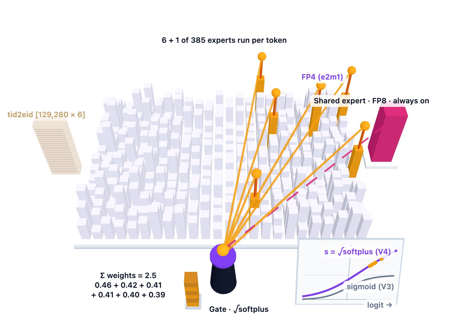
The 3D model above routes one token through a hash layer or a learned layer, with the bias on or off. Counts, formulas and dtypes are exact; its scores and table entries are synthetic.

Implementation notes: the gate in the reference code

• Gate.forward computes scores = linear(x.float(), weight.float()), then softplus(scores).sqrt() for score_func sqrtsoftplus. The code also supports softmax and sigmoid; the V4 configs select sqrtsoftplus.
• It keeps original_scores, adds the float32 bias (shape [n_routed_experts]) only for the topk call, and gathers the weights from original_scores. Renormalization applies for every scoring function except softmax; then weights *= route_scale.
• The routing weight is applied inside the expert, to the SwiGLU output before the down projection (§8.4). The shared expert is called without a weight.
• The gate takes the output of the layer’s ffn_norm, that is, the mHC-blended and normalized vector from §7.2.

8.3 Hash routing in the first three layers

In layers 0, 1 and 2, the router does not choose experts at all. A fixed table does: each token ID in the 129,280-entry vocabulary maps to a predetermined list of six experts. The report describes this as “Hash routing (Roller et al., 2021),” where “the target experts of each token” come from “a predefined hash function with regard to the input token ID.”

The reference code makes it concrete. In a hash layer, the gate holds a table tid2eid of shape $[129{,}280 \times 6]$, stored as int32 in the checkpoint and frozen (requires_grad=False). Routing a token is a lookup:

1. Who: read row token_id of the table, which gives six expert indices. No bias is involved; hash layers do not have one.
2. How much: compute the learned sqrt(softplus) scores for all experts as in §8.2, take the scores of those six, renormalize and multiply by the routing scale.

So hash layers are not uniform-weight layers: the table fixes who gets the token, and the learned gate still sets how much each of the six contributes. The animation below walks through both cases.

In the first three MoE layers a fixed table row (indexed by token id) decides which 6 of 384 experts run, but the learned gate still sets their weights; from layer 3 on, the gate's scores plus a selection-only bias pick the top-6. Token id, table entries and scores are illustrative. Open the full-size SVG.

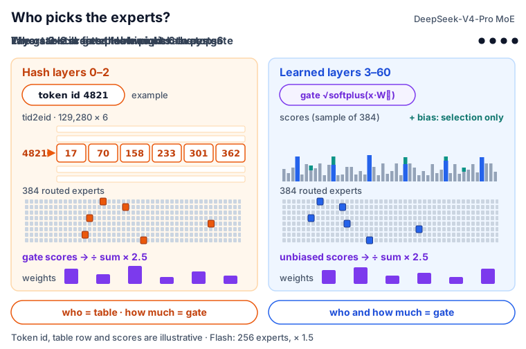
In plain terms: if row 4,821 of the table were $[17, 203, 88, 350, 5, 129]$ (a synthetic row), every occurrence of token 4,821 in layer 1 would go to those six experts, whatever its context. Their weights could still differ from one occurrence to the next, because the gate scores depend on the hidden state.

Why route by token ID at the bottom of the network? The sources do not say. Our reading is that in the first layers a token’s hidden state is still close to its embedding, so a learned router has little beyond the token’s identity to work with, and a fixed table gives perfectly predictable, stable routing there while keeping these layers sparse.

What the sources do not tell us

• How the table was built. The checkpoint ships tid2eid as data; neither the reference code nor the report shows the hash function, whether it balances load across experts, or whether a row can repeat an expert.
• How the hash-layer gate is trained. Its weights shape the routing weights, so it presumably receives gradients like any gate, but the training recipe for these layers is not described.
• Table size (derived): $129{,}280 \times 6$ int32 values, about 3.1 MB per hash layer.
• Gate.__init__ sets self.hash = layer_id < n_hash_layers with num_hash_layers = 3 in both configs. The multi-token-prediction layer has a layer index above 60 (Pro) or 42 (Flash), so it uses the learned router.

8.4 Inside an expert: SwiGLU with a clamp

Each expert, routed or shared, is a SwiGLU network. The input goes through two projections, a gate $W_1 h$ and an up projection $W_3 h$; the gate passes through SiLU and multiplies the up branch elementwise; a down projection $W_2$ maps the result back to width $d$. V4 adds one thing: before the multiplication, both branches are clamped.

\[u = \mathrm{clip}(W_3 h,\,-10,\,10),\qquad v = \min(W_1 h,\ 10),\qquad E(h) = W_2\big(g \cdot \mathrm{SiLU}(v) \odot u\big)\]

Here $g$ is the token’s routing weight for this expert from §8.2 ($g = 1$ for the shared expert). The code applies it before the down projection; because $W_2$ is linear, this is mathematically the same as weighting the output.

In plain terms: SiLU is at most about 9.9995 at input 10 and never below about −0.28, so with both clamps every entry of $\mathrm{SiLU}(v) \odot u$ stays within about ±100 (derived). Without the clamp, one unusually large activation could pass straight into the down projection.

The clamp is a training-stability fix that stays in the model. The report says loss spikes in V4 training were “consistently tied to outliers in the MoE layers” and that SwiGLU clamping “effectively eliminates outliers … without compromising performance.” It clamped the linear (up) part to $[-10, 10]$ and capped the gate at 10 throughout the training of both models. The config records the same value as swiglu_limit 10.0, and the reference inference code applies it in every routed and shared expert. §10.3 puts the clamp next to the other stability measure, anticipatory routing.

8.5 FP4 routed experts, FP8 shared expert

The routed experts are stored in FP4: 4-bit floats with 1 sign bit, 2 exponent bits and 1 mantissa bit (E2M1), packed two to a byte, with one 8-bit power-of-two scale per 32 weights. The shared expert stays in FP8 (E4M3 with one scale per 128 × 128 block), the checkpoint’s default format for quantized weights. At run time the FP4 weights are multiplied with FP8 activations.

By our count, one Pro expert takes about 35.1 MB in FP4 (scales included) instead of about 66.1 MB in FP8. Over all 61 layers, Pro’s routed experts come to roughly 822 GB, and Flash’s to roughly 147 GB over 43 layers.

What FP4 does not buy today is raw compute. The report is explicit: “the peak FLOPs for FP4 × FP8 operations are currently the same as FP8 × FP8 on existing hardware,” though they “can theoretically be implemented to be 1/3 more efficient on future hardware.” The present-day gain is memory: fewer bytes to store, and fewer bytes to read for each token (our reading: this matters most in decoding, where expert weights are read for only a handful of tokens at a time).

The FP4 weights come from quantization-aware training in the post-training stage, not from pre-training; §10.4 explains how.

Implementation notes: dtypes, sizes, and the fused MoE kernel

• Dtypes in the code. MoE.__init__ builds routed experts with torch.float4_e2m1fn_x2 when the config says expert_dtype: fp4; the shared expert is built without a dtype, so it takes the model default, FP8 E4M3 (quantization_config: e4m3, dynamic activation scales, ue8m0 scale format, 128 × 128 weight blocks). An FP4 Linear stores its weight as [out, in/2] packed bytes plus a float8_e8m0fnu scale of shape [out, in/32]; the forward pass quantizes activations to FP8 and calls fp4_gemm.
• Expert math precision. Expert.forward computes the gate and up branches, the clamp and SiLU in float32, then casts back before the down projection.
• Size arithmetic (derived): FP4 costs $0.5 + 1/32 = 0.53125$ bytes per weight with scales, so one Pro expert is $66{,}060{,}288 \times 0.53125 \approx 35.1$ MB (Flash: $25{,}165{,}824 \times 0.53125 \approx 13.4$ MB). Routed-expert totals: $61 \times 384$ experts (Pro) and $43 \times 256$ (Flash), main layers only.
• Fused MoE kernel (report §3.1). DeepSeek runs dispatch, the two expert matmuls and combine as one fused kernel that splits experts into “waves,” so that computing one wave, receiving tokens for the next and sending finished results overlap. Against strong non-fused baselines it reports 1.50–1.73× speedups for general inference and up to 1.96× for latency-sensitive cases such as reinforcement-learning rollouts, on NVIDIA GPUs and Huawei Ascend NPUs. The CUDA version is open-sourced as MegaMoE in DeepGEMM.
• A hardware rule of thumb from the same section. In V4-Pro each token-expert pair costs $6hd$ FLOPs but only $3h$ bytes of communication (FP8 dispatch, BF16 combine), so communication hides fully when compute-to-bandwidth $C/B \le 2d = 6{,}144$ FLOPs per byte, with $d = 3{,}072$ the expert width. The report also suggests replacing SwiGLU with a cheaper elementwise activation without exponentials or divisions.

9. Long Context: YaRN, KV Cache, and FLOPs vs V3.2

What does a million-token context actually cost a V4 model, and how is that cost served? This section puts the earlier mechanisms together into three answers: how positions stretch to 1,048,576 tokens, how many bytes the cache needs at that length, and how a server stores a cache whose layers all look different.

9.1 Positions to 1M

RoPE encodes a token’s position by rotating pairs of channels, each pair at its own speed. Fast pairs separate neighbors; slow pairs tell far-apart tokens apart. A model trained only on short sequences has never seen the slowest pairs turn very far, so it needs help before it can read positions it never trained on. YaRN is a standard fix: it slows down only the slow pairs and leaves the fast ones alone.

Both configs ask for the same YaRN setting:

Setting (config rope_scaling and neighbors)	V4-Pro	V4-Flash
type	yarn	yarn
original_max_position_embeddings	65,536	65,536
factor	16	16
beta_fast / beta_slow	32 / 1	32 / 1
max_position_embeddings	1,048,576	1,048,576
RoPE base in compressed layers (compress_rope_theta)	160,000	160,000
RoPE base in window-only layers (rope_theta)	10,000	10,000

In plain terms: 65,536 × 16 = 1,048,576, so the factor of 16 is exactly what turns a 64K design length into the advertised 1M window.

The reference code adds a twist that the paper never mentions (the report does not discuss YaRN at all). YaRN and the larger base apply only in layers that have a compressor. A layer whose compression ratio is 0, which attends only to its 128-token window, gets plain RoPE with base 10,000 and no YaRN. The code comment says so directly: “disable YaRN and use base rope_theta in pure sliding-window attention.”

That rule plays out differently in the two models, because their first two layers differ (§2.2):

• V4-Pro: all 61 main layers are CSA or HCA, so all 61 use YaRN with base 160,000.
• V4-Flash: layers 0 and 1 are window-only and use base 10,000 without YaRN; the other 41 use YaRN.
• Both: the MTP block’s entry in compress_ratios is 0, so it is window-only as well (derived from the configs and the code).

Our reading of why this is safe: a window-only layer never compares two positions more than 128 tokens apart, so it never meets a distance it did not see in training, and stretching its rotations would only blur them.

A tiny worked example shows what the factor of 16 does to V4’s 64 RoPE channels (32 rotating pairs). Running the reference code’s correction-range formula with base 160,000, 65,536 original positions, and betas 32 / 1 gives the split below (derived by us; the formula is in the code, the numbers are our evaluation of it):

Pairs (of 32)	Wavelength at base 160,000	What YaRN does
0–15	about 6 to 1,700 tokens	unchanged: these already cycle many times within 64K
16–24	in between	blended along a linear ramp
25–31	about 73,000 to 691,000 tokens	frequency divided by 16

The slowest pairs never complete one turn inside a 64K span. Dividing their speed by 16 maps the 1M range back onto angles a 64K design already covers. V4 does train on sequences up to 1M (see the details below), and the sources do not say at which stage the YaRN table was switched on.

Implementation notes

• Attention.__init__ picks the RoPE table per layer: original_seq_len, rope_theta = args.original_seq_len, args.compress_rope_theta when compress_ratio > 0, else 0, args.rope_theta (inference/model.py, around lines 475–482). precompute_freqs_cis applies YaRN only when original_seq_len > 0 (lines 200–228).
• One per-layer freqs_cis buffer is shared by the window keys, the compressor, and the indexer in that layer, so in a CSA or HCA layer even the 128 raw window tokens are rotated with the YaRN table.
• The YaRN formula is freqs = freqs / factor * (1 - smooth) + freqs * smooth, with smooth a ramp over pair index between find_correction_range(32, 1, 64, 160000, 65536) = (15, 25) by our evaluation.
• The reference attention uses a softmax scale of $512^{-1/2}$ (self.softmax_scale = self.head_dim ** -0.5); we found no YaRN attention-temperature (mscale) factor in V4’s model.py.
• Training lengths come from the paper: sequences grow from 4K to 16K, 64K, and finally 1M during pre-training (report §4.2.2). The paper does not connect these stages to the YaRN settings, and neither do we.

9.2 The cache at 1M

The KV cache is the memory a model keeps for every past token so it does not recompute them. V4 shrinks it in three ways at once: fewer entries per layer (compression), one 512-number entry shared by all heads (§3), and fewer bytes per number. The headline claim is the paper’s: by its estimate, at 1M tokens V4-Pro needs 10% of DeepSeek-V3.2’s KV cache and V4-Flash 7%.

We can rebuild those percentages from the configs with a simple byte model. Per layer, per stored entry:

• Main entry: 448 dims in FP8 plus 64 RoPE dims in BF16 = 448 + 128 = 576 bytes (ignoring the small FP8 scale bytes). The paper says this mixed format makes the cache “nearly half” the size of pure BF16 (512 × 2 = 1,024 bytes).
• Indexer key (CSA only): 128 dims in FP4 = 64 bytes (we ignore the small MXFP4 scale bytes).
• Window: 128 main entries per layer, a fixed 128 × 576 = 73,728 bytes no matter how long the context is.

Now count entries at $n$ = 1,048,576 tokens. A CSA layer stores $n/4$ = 262,144 entries, an HCA layer $n/128$ = 8,192. Worked through for V4-Pro (30 CSA layers, 31 HCA layers):

\[\underbrace{30 \times 262{,}144 \times (576+64)}_{\text{CSA: } 5.03\ \text{GB}} + \underbrace{31 \times 8{,}192 \times 576}_{\text{HCA: } 0.146\ \text{GB}} + \underbrace{61 \times 128 \times 576}_{\text{window: } 4.5\ \text{MB}} \approx 5.18\ \text{GB}\]

In plain terms: per layer and per token of context, a CSA layer costs (576 + 64) / 4 = 160 bytes and an HCA layer 576 / 128 = 4.5 bytes.

At 1M tokens (derived)	CSA layers	HCA layers	Window	Total	vs V3.2	Paper
DeepSeek-V3.2 (external assumption)	—	—	—	~50.4 GB	100%	—
V4-Pro	5.03 GB (30 layers)	0.146 GB (31)	4.5 MB (61)	~5.18 GB	10.3%	10% (“9.5x smaller”)
V4-Flash	3.52 GB (21 layers)	0.094 GB (20)	3.2 MB (43)	~3.62 GB	7.2%	7% (“13.7x smaller”)

The derived ratios land within rounding of the paper’s, so the byte model is a usable picture of where V4’s bytes live. Three things stand out:

1. CSA is almost the whole cache. About 97% of V4-Pro’s 5.18 GB sits in CSA layers, and roughly a tenth of that is indexer keys. Our reading: the 4:1 entries plus their indexer keys are the price of fine-grained sparse retrieval.
2. HCA is nearly free. Thirty-one layers that each see the whole million tokens cost 0.146 GB together.
3. The window is a constant. 4.5 MB for Pro, whether the prompt holds 1,000 tokens or a million.

The paper gives one more anchor: against a BF16 grouped-query attention baseline with 8 KV heads (GQA8) and head dimension 128 (a common attention layout), V4’s cache is “approximately 2%” at 1M. Our arithmetic agrees: that baseline stores 2 × 8 × 128 × 2 = 4,096 bytes per token per layer, which over 61 layers and 1M tokens is about 262 GB, and 5.18 / 262 ≈ 2.0% (derived, assuming the same depth).

Per-sequence KV cache from 8K to 1M tokens: DeepSeek-V3.2 (assumed 788 B/token/layer) reaches ~50 GB, while V4-Pro needs 5.2 GB and V4-Flash 3.6 GB (derived; the paper says 10% and 7%), almost all of it CSA entries and indexer keys. Switch to Keys / query to see what one query reads per layer: CSA tops out at 128 + top-k, while HCA reads all n/128 entries (8,320 at 1M) with no indexer scan.

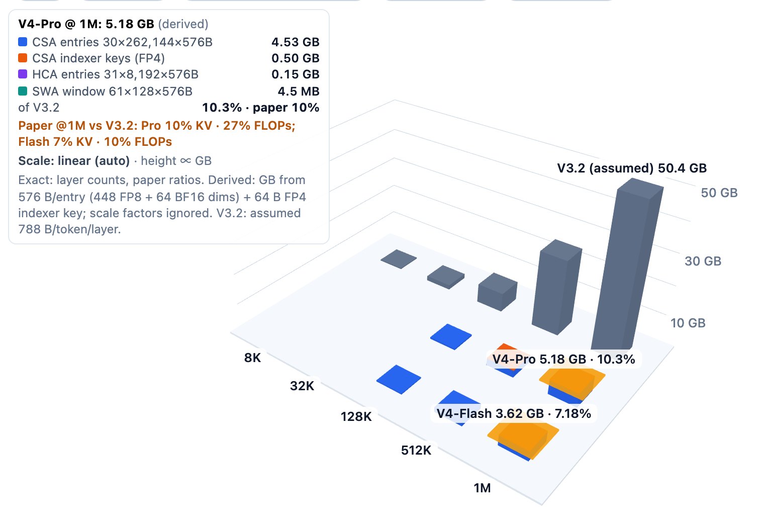
Where the numbers come from

• Exact (paper): 10% / 7% of V3.2’s KV cache at 1M (report abstract and §1; Figure 1 right reads “9.5x smaller” and “13.7x smaller”); mixed BF16/FP8 storage “nearly half” of BF16; indexer attention in FP4; “approximately 2%” of a BF16 GQA8, head-dim-128 baseline (report §2.3.4).
• Exact (configs): layer types from compress_ratios (Pro: 30 CSA + 31 HCA; Flash: 21 CSA + 20 HCA + 2 window-only), head_dim 512, qk_rope_head_dim 64, index_head_dim 128, sliding_window 128.
• Derived (ours): every GB figure above. Byte sizes follow the paper’s storage description and the reference code’s quantization (act_quant on the 448 non-RoPE dims; fp4_act_quant on the indexer keys). Decimal GB (10⁹ bytes).
• External assumption: the V3.2 reference of 788 bytes per token per layer (a 656-byte FP8 MLA latent plus a 132-byte indexer key, following the FlashMLA FP8 cache layout), over 61 layers. It is not stated in the V4 report; it matches the ~50 GB top of Figure 1’s KV axis.
• The reference code keeps the window and the compressed entries of a layer in one buffer of window_size + max_seq_len // compress_ratio rows of 512 (inference/model.py, line 473). The byte sizes above follow the paper’s storage format, not that buffer’s dtype.

9.3 Compute per token

Bytes are half the story; the other half is arithmetic per generated token. Here the paper gives two anchors at 1M context, measured in estimated “equivalent FP8 FLOPs” (the paper’s unit; it does not spell out the conversion): V4-Pro needs 27% of V3.2’s single-token FLOPs (“3.7x lower” in Figure 1) and V4-Flash 10% (“9.8x lower”). The paper stresses that Pro gets there “even” though it activates more parameters per token than V3.2.

The paper publishes those numbers only at 1M, without a breakdown, so we do not draw a FLOPs curve. What we can show exactly is how many cached entries one query reads in each kind of layer:

Layer type	Keys read per query (context $n$)	At $n$ = 1M	Source
Window-only	128	128	config
CSA, V4-Pro	128 + min(1,024, ⌊$n$/4⌋)	1,152	config index_topk 1,024
CSA, V4-Flash	128 + min(512, ⌊$n$/4⌋)	640	config index_topk 512
HCA (both)	128 + ⌊$n$/128⌋	8,320	derived from ratio 128
V3.2 DSA (for reference)	min(2,048, $n$)	2,048	external: V3.2 index_topk

In plain terms: a V4-Pro CSA layer at 1M reads 1,024 selected compressed entries plus the 128 newest raw tokens, and each selected entry summarizes 8 tokens at a stride of 4 (one new entry per 4 tokens).

Two cautions keep this table honest. First, an HCA layer at 1M reads more entries (8,320) than a V3.2 layer does (2,048), so entry counts alone do not explain the 27%. Second, a CSA layer’s lightning indexer still scores every compressed entry before it picks the top-k: 262,144 candidates at 1M, scored with 64 heads of 128 dims in FP4. V3.2’s indexer scores every token, four times as many candidates (from the V3.2 design, external to the V4 report). Our reading is that the savings come from all of these together: fewer candidates for the indexer, a smaller top-k (the paper names it as an efficiency choice for short and medium texts), cheap dense attention in HCA, and FP4/FP8 arithmetic.

9.4 Serving the heterogeneous cache

A standard inference server cuts every layer’s cache into equal pages, one page per fixed number of tokens. V4 breaks that habit: a CSA layer adds one entry every 4 tokens, an HCA layer one every 128, and every layer also keeps a 128-token window that slides. The paper’s answer is to split the cache into two pools, one that grows with the context and one that does not.

The paper names two reasons why PagedAttention-style paging does not fit as is: layers follow different cache policies (the sliding window evicts, compressed entries do not), and fast attention kernels need aligned blocks. Its design:

1. A block cache for compressed entries. Each block covers a multiple of lcm(4, 128) = 128 original tokens. For one 128-token block, a CSA layer stores 32 entries (plus their indexer keys) and an HCA layer stores 1 (derived from the ratios). The sparse-attention kernel was co-designed so that blocks of any such size run at full speed.
2. A state cache for everything that is still in motion. Each request gets one fixed-size slot holding the window’s last 128 KV entries and the “uncompressed tail”: tokens that have arrived but do not yet fill a compression block. The paper treats this slot like the state of a state-space model, which depends only on the current position, and pre-allocates a fixed pool of such slots.

Take the 1,000-token V4-Pro prompt from §4.3 (derived). The block cache receives the compressed entries: 250 per CSA layer and 7 per HCA layer. The state slot holds what is still moving: every layer’s window (tokens 872 to 999), the 104 pending tokens of each HCA layer, and, for each CSA layer, only the last 4-token block that the overlapping compressor reuses for the next entry.

The same split shapes the on-disk prefix cache, which lets requests that share a long prefix skip prefill:

• Compressed entries (CSA and HCA) are all written to disk. A hit reuses them up to the last complete compression block; the incomplete tail block is recomputed.
• Window entries exist in every layer and are not compressed, so storing them for every token would take about 8 times the space of the compressed entries (paper). The paper offers three options (SWA stands for sliding-window attention): Full SWA Caching (store all of them; no recomputation but a write-heavy SSD pattern), Periodic Checkpointing (store the last 128 window entries every $p$ tokens, then recompute from the nearest checkpoint), and Zero SWA Caching (store none and recompute).

Zero SWA Caching works because a token’s window entry in one layer depends only on the previous 128 tokens of the layer below. Recomputing the last $n_\text{win} \cdot L$ tokens on top of the cached compressed entries therefore restores every window. That is 128 × 61 = 7,808 tokens for V4-Pro and 128 × 43 = 5,504 for V4-Flash (derived), a fixed cost however long the shared prefix is.

Implementation notes

• The pending tail lives in each compressor’s FP32 kv_state and score_state buffers (§4.3), whose sizes do not depend on the context length: [·, 8, 1024] for a CSA main compressor, [·, 8, 256] for its 128-dim indexer compressor, and [·, 128, 512] for an HCA compressor (inference/model.py, lines 303–304).
• Our check of the “8 times” figure, assuming all window entries are written for every token: per token, V4-Pro’s windows hold 61 × 576 = 35,136 bytes and its compressed main entries 30 × 144 + 31 × 4.5 ≈ 4,460 bytes, a ratio of about 7.9 (derived; including indexer keys gives about 7.1).

How well do the models actually use a million tokens? The model cards report two 1M-token tests in their reasoning-mode comparison (Max is the highest-effort mode, §11.4): MRCR 1M, which measures in-context retrieval, and CorpusQA 1M, which the paper calls “similar to real scenarios.”

1M-token benchmark (card)	V4-Flash Max	V4-Pro Max
MRCR 1M	78.7	83.5
CorpusQA 1M	60.5	62.0

In the card’s comparison with frontier models, Gemini-3.1-Pro High scores 76.3 and 53.8 on the same two tests and Opus-4.6 Max 92.9 and 71.7. That matches the paper’s summary for MRCR (ahead of Gemini-3.1-Pro, behind Opus-4.6); for CorpusQA it notes Pro beats Gemini-3.1-Pro.

10. Training: Data, Muon, Stability, and FP4 QAT

How do you train a trillion-parameter model that reads a million tokens without it falling over? The report’s answer has four parts: more and longer data, a different optimizer (Muon), two tricks that stop loss spikes, and a last stage that teaches the model to live with 4-bit experts.

10.1 Data and the pre-training schedule

The pre-training corpus builds on DeepSeek-V3’s data and comes to “more than 32T tokens”: V4-Flash saw 32T and V4-Pro 33T. The report lists what changed:

• Cleaner web data. Filters remove batched auto-generated and templated pages, to reduce the risk of model collapse from training on machine-made text.
• Agentic data in mid-training, added to strengthen coding; math and code remain core components.
• A larger multilingual corpus, aimed at long-tail knowledge across cultures.
• Long documents, with priority on scientific papers, technical reports, and similar material.
• Same tokenizer family. The vocabulary stays at 128K (the configs list 129,280 entries), with a few new special tokens for building contexts. Token-splitting and Fill-in-Middle (FIM) are inherited from V3.
• Packing with sample-level attention masking. Documents from different sources are packed into one training sequence to avoid truncation, and, new compared with V3, attention is masked per sample.

In plain terms: if a 4K training sequence holds a 3,000-token paper followed by a 1,096-token code file, sample-level masking stops the code tokens from attending to the paper. Our reading is that this matters more for V4 than for V3, because each packed document is also compressed on its own; the paper’s context-parallelism section notes that every packed sequence is compressed independently, with leftover tokens that do not fill a block discarded.

The two models then follow the same schedule with different numbers:

Pre-training setup (paper §4.2.2)	V4-Flash	V4-Pro
Tokens	32T	33T
Batch size (tokens)	ramps up to 75.5M, then held	ramps up to a maximum of 94.4M
Learning rate	2,000-step warmup, 2.7 × 10⁻⁴, cosine decay to 2.7 × 10⁻⁵ near the end	“largely the same” schedule, 2.0 × 10⁻⁴ to 2.0 × 10⁻⁵
Sequence length	4K → 16K → 64K → 1M	4K → 16K → 64K → 1M
Dense-attention warmup	first 1T tokens	“a longer stage” (no number given)
Sparse attention	introduced at 64K, after a short lightning-indexer warmup	same two-stage method
MoE balancing	bias update speed 0.001; sequence-wise balance loss weight 0.0001	same
MTP loss weight	0.3, then 0.1 once the learning rate starts to decay	same

The dense-then-sparse recipe mirrors how DeepSeek-V3.2 introduced DSA, which the GLM-5.3 post walks through in its §5.4. The V4 report says only that it warms up the indexer briefly before switching on sparsity; it does not state the indexer’s training loss, so we do not guess it.

10.2 Muon with hybrid Newton-Schulz

Muon is an optimizer for weight matrices. Adam-style optimizers scale each number of the gradient separately; Muon instead looks at a matrix’s update as a whole and replaces it with the nearest orthogonal matrix, so every direction the update points in moves by the same amount. V4 uses Muon for most of its weights, citing faster convergence and better stability. (The GLM-5.3 post §3.6 discusses how Muon interacts with attention design in GLM-5.)

Who gets which optimizer. AdamW keeps four groups: the embedding, the prediction head, the static biases and gating factors of mHC, and all RMSNorm weights. Everything else, including every expert matrix and every attention projection, is updated by Muon.

The paper’s Algorithm 1, for each “logically independent” weight $W \in \mathbb{R}^{n \times m}$ (each expert counts as its own set of matrices):

1. Take the gradient $G_t$ and update the momentum buffer: $M_t = \mu M_{t-1} + G_t$, with $\mu$ = 0.95.
2. Orthogonalize the Nesterov-style blend: $O’_t = \text{HybridNewtonSchulz}(\mu M_t + G_t)$.
3. Rescale: $O_t = O’_t \cdot \sqrt{\max(n,m)} \cdot \gamma$, so the update’s RMS is 0.18.
4. Apply weight decay and the step: $W_t = W_{t-1}(1 - \eta\lambda) - \eta O_t$, with $\lambda$ = 0.1.

Why $\sqrt{\max(n,m)}$? An orthogonalized $n \times m$ matrix has all singular values equal to 1, which works out to an RMS of $1/\sqrt{\max(n,m)}$ per entry. Multiplying by $\sqrt{\max(n,m)}$ brings that to 1, and $\gamma$ brings it to 0.18 (our derivation of the paper’s stated target). For V4-Pro’s query down-projection, a 7,168 × 1,536 matrix, the factor is $\sqrt{7{,}168} \approx 84.7$. Matching the RMS is what lets Muon reuse the AdamW learning rate.

Orthogonalizing exactly would need a singular value decomposition (SVD), which is too slow to run on every matrix at every step. Newton-Schulz iterations approximate it with matrix multiplications only. Normalize $M_0 = M / \lVert M \rVert_F$ so no singular value exceeds 1, then repeat

\[M_k = a\,M_{k-1} + b\,(M_{k-1}M_{k-1}^{\top})\,M_{k-1} + c\,(M_{k-1}M_{k-1}^{\top})^{2}\,M_{k-1}.\]

Each step applies the polynomial $f(\sigma) = a\sigma + b\sigma^3 + c\sigma^5$ to every singular value $\sigma$ and leaves the singular vectors alone. V4’s “hybrid” version runs 10 steps in two stages:

Steps	$(a, b, c)$	Job
1–8	(3.4445, −4.7750, 2.0315)	push small singular values up fast, toward 1
9–10	(2, −1.5, 0.5)	settle them precisely at 1

A tiny worked example (our simulation of the scalar polynomial): start with a singular value of 0.01. The first eight steps take it to 0.034, 0.118, 0.40, 1.09, then it bounces between about 0.70 and 1.12, ending at 1.086. The last two steps give 1.006 and then 1.000. The second polynomial has $f(1) = 1$ and slope $f’(1) = 2 - 4.5 + 2.5 = 0$, which is why it pins values at exactly 1, while the first one is fast from far away but never settles.

No QK-Clip. As §3.2 noted, V4 does not pair Muon with QK-Clip. Instead, its attention applies RMSNorm directly to the queries and the KV entries, which the paper says prevents exploding attention logits on its own.

Hyper-parameters and infrastructure

• Values (paper §4.2.2): AdamW $\beta_1$ = 0.9, $\beta_2$ = 0.95, $\varepsilon$ = 10⁻²⁰, weight decay 0.1. Muon momentum 0.95, weight decay 0.1, update RMS rescaled to 0.18. The same for Flash and Pro. (The report §4.2.2 list of AdamW modules omits mHC; report §2.4 includes the mHC static biases and gating factors.)
• Lineage: weight decay on Muon parameters, the Nesterov trick, and RMS rescaling follow Liu et al. (2025, Moonlight); the two-stage Newton-Schulz is V4’s change.
• Muon meets ZeRO (report §3.4.1). Muon needs whole matrices, while ZeRO shards optimizer state. For dense weights, V4 limits the ZeRO group size and assigns whole matrices to ranks with a knapsack-style packing (in their setup each rank manages no more than five matrices, and padding buckets to equal size typically costs under 10% extra memory); past that limit the update is computed redundantly. Expert matrices are optimized independently: all experts’ down, then up and gate matrices are flattened across layers and padded so that no matrix is split.
• Same-shape parameters are merged so Newton-Schulz runs batched; Newton-Schulz is stable in BF16 matrix multiplies.
• MoE gradients are stochastically rounded to BF16 for data-parallel synchronization, halving traffic, and reduce-scatter is replaced by an all-to-all plus a local FP32 sum.

10.3 Stability: anticipatory routing and SwiGLU clamping

The V4 training runs hit loss spikes, and rolling back to an earlier checkpoint only postponed the next one. The team traced the spikes to outliers inside the MoE layers and found that routing itself seemed to amplify them. They fixed it from two sides: break the feedback loop through the router, and cap the outliers directly. The paper is candid that “a comprehensive theoretical understanding” of why these work is still open.

Anticipatory Routing. At step $t$ the network computes features with its current parameters $\theta_t$, but the routing indices (which experts each token goes to) come from older parameters $\theta_{t-\Delta t}$. In practice:

1. At step $t - \Delta t$, the trainer already fetches the batch for step $t$ and runs one extra forward pass to compute and cache its routing indices.
2. At step $t$, the MoE layers use those cached indices instead of routing with the current router.
3. The extra forward pass is overlapped with expert-parallel communication, which bounds the wall-clock overhead at about 20% while the mode is on.
4. The mode is not always on. An automatic detector triggers a short rollback when a loss spike appears, runs with anticipatory routing for a while, then returns to normal training.

Our reading: if the router and the experts update in the same step, a small outlier can shift routing, which sends the expert more of the tokens that produced the outlier, which grows it further. Using slightly stale routing decisions cuts that loop. Because the mode only runs around spikes, the paper reports “negligible overall additional training overhead.”

SwiGLU clamping. Each expert computes $\text{SiLU}(\text{gate}) \odot \text{up}$. Throughout training of both models, the linear (“up”) part was clamped to $[-10, 10]$ and the gate capped from above at 10, which is the configs’ swiglu_limit of 10.0. The reference code applies it in every expert, routed and shared:

up = torch.clamp(up, min=-self.swiglu_limit, max=self.swiglu_limit)
gate = torch.clamp(gate, max=self.swiglu_limit)
x = F.silu(gate) * up

With both clamps, each element of the product stays within roughly ±100, as §8.4 works out (derived). The paper reports that clamping “effectively eliminates outliers” without hurting quality.

10.4 FP4 quantization-aware training

The released models store their routed experts in 4-bit floating point (§8.5). A model trained in higher precision loses some accuracy when its weights are rounded that hard, so V4 adds QAT: during post-training, the forward pass already uses the rounded weights, and the model learns to cope with them. QAT runs in post-training only; the paper does not describe FP4 QAT in pre-training.

FP4 here means MXFP4, a block format: E2M1 values (§8.5) in which every 1 × 32 run of values shares a scale. V4 applies it to two places:

1. MoE expert weights, a major consumer of GPU memory.
2. The query-key path of the CSA lightning indexer, whose activations are cached, loaded, and multiplied entirely in FP4. In the same QAT stage the index scores are stored in BF16 instead of FP32, which the paper says doubles the speed of the top-k selector while keeping a 99.7% recall of the selected KV entries.

The expert-weight recipe reuses the existing FP8 training stack:

1. The optimizer keeps FP32 master weights.
2. The forward pass quantizes them to FP4, then dequantizes to FP8 (E4M3) and computes in FP8.
3. The backward pass computes gradients with respect to those same FP8 weights and passes them straight to the FP32 masters, the straight-through estimator (STE). No transposed weights need re-quantizing.
4. Rollouts in reinforcement learning, and inference, skip the simulation and run native FP4 weights, so sampling behaves exactly like deployment. The indexer’s QK path is handled the same way.

Step 2 sounds lossy, but the paper argues it is exact. FP8 E4M3 has two more exponent bits than FP4 E2M1, so as long as the 1 × 32 FP4 scales inside one 128 × 128 FP8 block do not differ by more than some ratio, the FP8 exponent can absorb the finer scales and every FP4 value is represented exactly. The team checked empirically that the current weights meet that condition. In plain terms (our illustration): if two 32-value runs in one FP8 block have scales 1 and 1/8, a value of 1.5 in the second run becomes 0.1875, which E4M3 stores exactly; only a very large spread of scales inside one block would fall outside FP8’s range.

As §8.5 noted, the gain is memory, not compute: on current hardware FP4 × FP8 runs at the same peak FLOPs as FP8 × FP8.

Implementation notes

• Reference inference code: routed experts are float4_e2m1fn_x2 tensors, two FP4 values per byte (inference/model.py, line 623); the shared expert is not FP4. On the indexer side, the compressed indexer keys and the indexer queries go through a Hadamard rotation and fp4_act_quant with block size 32 (lines 368–370 and 414–416).
• Miles, the open training implementation (§13), has FP8 activation QAT (fp8_simulate_qat, straight-through backward) but we found no FP4 expert-weight QAT in it, and its indexer compressor simulates FP8 with block 128 where the reference code uses FP4 with block 32.
• The paper’s post-training applies QAT to teacher and reference models too, so every model in the distillation pipeline adapts to the same rounding.

10.5 Systems box

The report spends a long chapter on infrastructure. Most of it is beyond this post, but five pieces explain how the architecture above becomes trainable at all. (The fused MoE kernel, MegaMoE, is covered with the MoE layer in §8.)

Piece (paper section)	Problem	What V4 does
TileLang kernels (§3.2)	hundreds of small PyTorch operators, each with CPU launch overhead	fused kernels written in the TileLang language; host-side code generation cuts per-call CPU validation from tens or hundreds of microseconds to under 1 μs; an SMT solver (Z3) helps the compiler reason about integer index math at a cost of a few seconds of compile time; fast-math is off by default for bitwise reproducibility
Batch-invariant, deterministic kernels (§3.3)	results that change with batch size or thread timing make training and inference disagree	decode attention without split-KV, using a single-SM and a multi-SM kernel with the same accumulation order; cuBLAS replaced end to end by DeepGEMM, split-k avoided in most cases; deterministic sparse-attention and MoE backward passes instead of atomic adds, and a deterministic split-k reduction for mHC’s small matmul
mHC implementation (§3.4.2)	four residual streams raise activation memory and the traffic between pipeline stages	fused kernels, selective recomputation (most hidden states and all normalized inputs are recomputed; compute-heavy operations are not), and an adjusted DualPipe 1F1B overlap hold mHC’s wall-time overhead to 6.7% of an overlapped 1F1B pipeline stage
Context parallelism for compressed attention (§3.4.3)	a compression block can straddle two GPUs, and packed sequences compress to uneven lengths	two stages: each rank sends its last $m$ uncompressed KV entries to the next rank, which compresses to a fixed $s/m + 1$ entries with padding; an all-gather plus a fused select-and-pad then assembles all compressed entries
Tensor-level activation checkpointing (§3.4.4)	module-level checkpointing is too coarse, and hand-writing a layer’s backward pass gives up automatic differentiation	developers mark individual tensors; a TorchFX trace finds the minimal subgraph to recompute each one before its gradient is needed, with no extra overhead versus hand-written recomputation

Our reading of the common thread: V4’s tricks (top-k selection, compression with lookback, four residual streams) all create places where tiny numerical differences or uneven shapes could break reproducibility, so the infrastructure leans hard on deterministic, shape-aware kernels.

11. Post-Training and Reasoning Modes

How does a pretrained V4 base model become the chat model with three thinking levels? DeepSeek first trains a set of separate specialists, one per domain and reasoning budget. It then distills all of them into a single student that learns from its own samples. That second step replaces the mixed reinforcement-learning stage DeepSeek used for V3.2.

11.1 Specialists first, then one student

The technical report describes a pipeline that “largely mirrored” DeepSeek-V3.2’s, with one substitution. The order is:

1. Specialists. Each domain specialist is fine-tuned (supervised fine-tuning, SFT) and then trained with reinforcement learning (RL) on domain-specific prompts and rewards. The RL algorithm is GRPO (Group Relative Policy Optimization), with hyper-parameters “closely aligned” with DeepSeek’s earlier work.
2. Specialists per reasoning effort. Reasoning budget is also a specialist axis. DeepSeek trains distinct specialists under different RL settings, each with its own length penalty and context window, so they learn to think for different lengths (§11.4).
3. One student. Multi-teacher On-Policy Distillation (OPD) merges “more than ten” teachers into the final model. The report says the mixed RL stage was “entirely replaced” by OPD.

A judge that is also the actor. Easy-to-check tasks (math answers, unit tests) use rule-based verifiers. For hard-to-verify tasks, V4 drops the usual scalar reward model. DeepSeek writes rubric-guided RL data and scores trajectories with a Generative Reward Model (GRM), a model that writes out its judgment. The report then applies RL to the GRM itself: “the actor network natively functions as the GRM,” so judging and generating are optimized together. The report says this needs “only a minimal set of diverse human annotations.”

11.2 On-policy distillation, with the whole vocabulary

In OPD the student writes the trajectories, and the teacher relevant to each task grades every token of them. With $N$ expert teachers $\pi_{E_1}, \dots, \pi_{E_N}$, the report’s objective (its Eq. 29) is

\[\mathcal{L}_{\text{OPD}}(\theta) = \sum_{i=1}^{N} w_i \, D_{\text{KL}}\!\left(\pi_\theta \,\Vert\, \pi_{E_i}\right)\]

Here $\pi_\theta$ is the student, $w_i$ is a per-teacher weight (“typically determined by the relative importance of the expert”), and the KL runs from student to teacher, the reverse direction. Reverse KL is an average over the student’s own distribution, so the training text has to come from the student; that is what makes it on-policy. In plain terms: the student answers a math prompt itself, and the math teacher tells it, token by token, how its whole next-token distribution should have looked.

The report’s second choice concerns how that KL is computed. Earlier OPD work usually keeps only the token that was actually sampled and uses $\log \pi_{E_i}(y_t) - \log \pi_\theta(y_t)$ as a per-token advantage inside an RL loss. DeepSeek reports that this estimate has “high variance” and “often causes training instability,” so V4 computes the KL over the full vocabulary at every position.

A toy example shows the difference. Take a 4-token vocabulary, a student distribution $p = (0.5, 0.3, 0.1, 0.1)$ and a teacher $q = (0.7, 0.1, 0.1, 0.1)$:

What is computed	Value (nats)
Full-vocabulary reverse KL, $\sum_v p_v \ln (p_v / q_v)$	$0.5 \ln\frac{5}{7} + 0.3 \ln 3 \approx 0.161$
One-sample estimate if the student sampled token 1	$\ln\frac{0.5}{0.7} \approx -0.336$
One-sample estimate if it sampled token 2	$\ln\frac{0.3}{0.1} \approx +1.099$

Weighted by how often the student samples each token, the one-sample numbers average to the same 0.161 (tokens 3 and 4 contribute 0). But any single one can be negative or about seven times too large. The full-vocabulary loss gives the exact value at every position. The price is memory: the real vocabulary has 129,280 entries, for every token, for each teacher that scores it.

How DeepSeek makes full-vocabulary OPD affordable

The report (§5.2) lists the infrastructure behind OPD with more than ten teachers, each “potentially comprising trillions of parameters”:

• Teachers live off-GPU. All teacher weights sit in centralized distributed storage and are loaded on demand with ZeRO-like sharding.
• Cache hidden states, not logits. Writing out logits for a vocabulary above 100k for every teacher is “prohibitive, even when spooled to disk.” DeepSeek caches only each teacher’s last-layer hidden state and recomputes the logits through that teacher’s prediction head at training time. By our count from the V4-Pro config, a hidden state has 7,168 values against 129,280 logits, about 18× less to store per token (derived).
• One teacher head at a time. Training samples are ordered by teacher index, so each head is loaded once per mini-batch and at most one sits in device memory. Loading and offloading run asynchronously.
• Exact KL in a kernel. The teacher–student KL is computed by a dedicated TileLang kernel.

Toy example: the 4-token numbers above are ours, chosen to show the variance argument; they are not from the report.

11.3 Rollouts that survive preemption

RL and OPD both need long student rollouts, and DeepSeek runs them on a cluster where any job can be preempted and hardware fails. The report’s rollout service keeps a token-granular write-ahead log (WAL) per request: every new token is appended the moment it is generated.

• On preemption, the engine pauses and saves the KV cache of unfinished requests. On resumption it continues decoding from the WAL and the saved cache.
• After a fatal hardware error, it re-runs prefill over the logged tokens to rebuild the KV cache, then continues.

Why not simply restart unfinished requests? The report calls that “mathematically incorrect” because it introduces length bias. Short responses are more likely to finish before an interruption, so restarting interrupted ones replaces long answers with fresh samples, and the finished set tilts toward short answers. In plain terms: if a 2,000-token answer and a 40,000-token answer start together and a preemption hits at token 10,000, only the long one is thrown away.

A batch-invariant, deterministic stack could instead regenerate interrupted requests with the same sampler seed, but that re-runs the whole decode; the WAL avoids the cost.

For million-token RL, the report also splits rollout data into light metadata (loaded in full for global shuffling and packing) and heavy per-token fields (streamed through a shared-memory loader and freed after each mini-batch).

11.4 Three reasoning modes

Both V4-Pro and V4-Flash ship with three modes, built from the effort-specific specialists of §11.1. Table 2 of the report and the model cards describe them:

Mode	Character	Response format
Non-think	“Fast, intuitive” answers for routine tasks	</think> summary
Think High	“Conscious logical analysis, slower but more accurate”	<think> thinking </think> summary
Think Max	“Push reasoning to its fullest extent”	special system prompt + <think> thinking </think> summary

At inference time, Think Max differs from Think High by an instruction prepended to the system prompt (report Table 3). It begins: “Reasoning Effort: Absolute maximum with no shortcuts permitted.” The rest asks the model to decompose the problem, stress-test its logic against edge cases, and write out every rejected hypothesis. The preview cards recommend temperature = 1.0, top_p = 1.0 for local deployment, and a context window of at least 384K tokens for Think Max.

The later -0731 and -0813 cards (§12.2) rename the knob: reasoning_effort takes low, high, or max. They recommend top_p = 0.95 for agentic work (1.0 otherwise) and a maximum output length of 384K tokens for high and max. The cards do not map the old names to the new ones; reading low as the successor of Non-think is our interpretation.

What do the modes buy? The preview card’s mode table, excerpted (higher is better):

Benchmark	Flash Non-think	Flash High	Flash Max	Pro Non-think	Pro High	Pro Max
HLE	8.1	29.4	34.8	7.7	34.5	37.7
GPQA Diamond	71.2	87.4	88.1	72.9	89.1	90.1
LiveCodeBench	55.2	88.4	91.6	56.8	89.8	93.5
Codeforces (rating)	–	2816	3052	–	2919	3206
HMMT 2026 Feb	40.8	91.9	94.8	31.7	94.0	95.2
MRCR 1M	37.5	76.9	78.7	44.7	83.3	83.5
SimpleQA-Verified	23.1	28.9	34.1	45.0	46.2	57.9
BrowseComp	–	53.5	73.2	–	80.4	83.4

Two patterns stand out. First, thinking is most of the score on reasoning tasks: Pro’s HLE goes from 7.7 to 34.5 to 37.7. Second, Flash at Max roughly matches Pro at High on reasoning (HLE 34.8 vs 34.5, LiveCodeBench 91.6 vs 89.8, Codeforces 3052 vs 2919), as the card says, but not on knowledge: Flash-Max’s SimpleQA-Verified score (34.1) is below even Pro’s Non-think score (45.0). The report attributes the knowledge gap to parameter count (“larger parameter counts facilitate greater knowledge retention”); reasoning, by contrast, tracks the thinking budget.

11.5 Tool calls, kept reasoning, and quick instructions

Three interface changes ship with the post-trained models. None touches the architecture, but each changes what an application sends and gets back.

DSML tool calls. V4 introduces a dedicated DSML special token (the tag prefix in the block below) and an XML-style tool-call block (report Table 4). String parameters are passed as-is with string="true"; numbers, booleans, arrays, and objects are passed as JSON with string="false":

<|DSML|tool_calls>
<|DSML|invoke name="get_weather">
<|DSML|parameter name="city" string="true">Hangzhou</|DSML|parameter>
<|DSML|parameter name="days" string="false">3</|DSML|parameter>
</|DSML|invoke>
</|DSML|tool_calls>

The tool name and arguments here are our example; the tags are from the report. DeepSeek reports that the XML format “effectively mitigates escaping failures and reduces tool-call errors.” In plain terms: a code snippet passed as a string no longer has to survive JSON escaping of every quote and newline.

Reasoning that survives user turns. V3.2 kept its reasoning across tool-result rounds but dropped it when a new user message arrived. V4 keeps all reasoning for the whole conversation in tool-calling scenarios, across user turns, and still drops it in plain chat. The report notes that frameworks which simulate tools through user messages (it names Terminus) may not trigger the tool-calling path, and it still recommends non-think mode there.

Quick Instruction tokens. Chatbots run small side tasks before answering: should this trigger a web search, what is the query, which domain is it? Instead of a separate small model that has to prefill the prompt again, V4 appends a dedicated special token to the existing sequence and reuses the KV cache already computed. Some of these tasks can run in parallel, which the report says “significantly reduces” time to first token. The seven tokens and where they go (report Table 5):

<|action|>          search the web, or answer directly?   ...<|User|>{prompt}<|Assistant|><think><|action|>
<|title|>           conversation title                    ...<|Assistant|>{response}<|end_of_sentence|><|title|>
<|query|>           search queries for the prompt         ...<|User|>{prompt}<|query|>
<|authority|>       how authoritative must sources be?    ...<|User|>{prompt}<|authority|>
<|domain|>          domain of the prompt                  ...<|User|>{prompt}<|domain|>
<|extracted_url|>   fetch and read each URL? (pair)       ...<|User|>{prompt}<|extracted_url|>{url}<|read_url|>
<|read_url|>        (closes the pair)

Implementation notes

• The model cards ship no Jinja chat template. An encoding folder provides encode_messages(messages, thinking_mode="thinking") and parse_message_from_completion_text, with OpenAI-compatible messages that carry reasoning in a reasoning_content field. The -0731 and -0813 cards add reasoning_effort="max" to the same call.
• The tool-call system prompt also requires that, in thinking mode, the complete reasoning appears inside <think>…</think> before any tool call.

11.6 Where V4-Pro-Max stands

The preview card compares V4-Pro at Think Max with closed and open frontier models. An excerpt, with the best score in each row of the full table in bold:

Benchmark	Opus-4.6 Max	GPT-5.4 xHigh	Gemini-3.1-Pro High	DS-V4-Pro Max
LiveCodeBench	88.8	–	91.7	93.5
Codeforces (rating)	–	3168	3052	3206
Apex Shortlist	85.9	78.1	89.1	90.2
GPQA Diamond	91.3	93.0	94.3	90.1
HLE	40.0	39.8	44.4	37.7
SimpleQA-Verified	46.2	45.3	75.6	57.9
MRCR 1M	92.9	–	76.3	83.5
Terminal Bench 2.0	65.4	75.1	68.5	67.9
SWE Verified	80.8	–	80.6	80.6

The full table also includes Kimi K2.6 and GLM-5.1; in it, V4-Pro-Max is the top score only on LiveCodeBench, Codeforces, and Apex Shortlist.

These are preview numbers. The agentic scores moved a lot in the later releases, on newer benchmark versions, which is where §12 picks up.

12. After the Preview

The first V4 weights were labeled a preview. Later repositories added a speculative-decoding module, then official Flash and Pro releases with much stronger agent scores, then a first vision model. All of them keep the V4 backbone. DeepSeek-V4.1-Flash, the newest, is a different model that pushes KV compression further.

12.1 DSpark: the same checkpoint with a drafter attached

Decoding one token at a time leaves a big model limited by memory bandwidth. Speculative decoding lets a small, cheap module guess several tokens ahead, and the big model checks the whole guess in one forward pass. Correct guesses are kept, so several tokens can come out of one big-model step.

The DeepSeek-V4-Pro-DSpark card is explicit: it is “not a new model. It is the same checkpoint with an additional speculative decoding module attached.” It points to DeepSeek’s DeepSpec repository for the method. The config adds four keys and two extra ratio-0 entries; nothing else changes:

Config key	V4-Pro (DSpark, -0813)	V4-Flash (-0731, Vision-Exp)
dspark_block_size	5	5
dspark_target_layer_ids	[58, 59, 60]	[40, 41, 42]
dspark_markov_rank	512	256
dspark_noise_token_id	128799	128799
Trailing window-only (ratio 0) entries in compress_ratios	3 (64 entries for 61 layers)	3 (46 entries for 43 layers)

The target layers are the last three main layers of each model. The preview configs had one trailing ratio-0 entry, for the MTP block; the DSpark configs have three. Our reading is that the drafter consists of three window-only blocks that read hidden states from the last three layers.

The V4 report does not describe DSpark. The V4.1-Flash report describes its own DSpark drafter; we assume the V4 drafters follow the same design (our interpretation): three Transformer blocks with a 128-token window; one forward pass produces base logits for 5 draft positions in parallel; a lightweight “Markov head” models dependencies among the draft tokens; and a confidence head predicts how likely each prefix is to be accepted.

A scheduler combines those estimates with profiled engine throughput to choose how many tokens to verify per request. The report also says DSpark is trained after backbone pretraining with the backbone frozen, and that it speeds up RL and OPD rollouts as well as serving.

Serving flags from the cards

• vLLM (Pro-DSpark, Flash-0731, Pro-0813): --speculative-config '{"method":"dspark","num_speculative_tokens":7,"draft_sample_method":"greedy"}'. The cards give an example “on a single 4×GB300 node” with --kv-cache-dtype fp8 --block-size 256 --data-parallel-size 4 --enable-expert-parallel --moe-backend deep_gemm_mega_moe --attention-config '{"use_fp4_indexer_cache": true}'.
• vLLM (Vision-Exp): "num_speculative_tokens":3, "draft_sample_method":"probabilistic", "enable_adaptive_verification":true.
• SGLang: --speculative-algorithm DSPARK with no separate draft-model path, because “target and draft weights … come from the same checkpoint.”
• Open detail: the configs say block size 5 while the vLLM examples speculate 7 or 3 tokens. The sources do not explain how the two relate.
• num_nextn_predict_layers stays 1 in the Pro-DSpark, -0731, and -0813 configs but is 3 in Vision-Exp. The sources do not explain the difference.

12.2 Flash-0731 and Pro-0813: the official releases

DeepSeek-V4-Flash-0731 is “the official release of DeepSeek-V4-Flash, superseding the preview version,” with “the same model structure as DeepSeek-V4-Flash-DSpark.” DeepSeek-V4-Pro-0813 does the same for Pro: “built on the DeepSeek-V4-Pro (Preview) model structure, with a DSpark speculative decoding module attached.” The suffixes suggest July 31 and August 13 by DeepSeek’s past naming, but the cards never state a date. Both cards still cite the V4 report, and neither describes a new training recipe.

What changed is agent performance. The -0813 card puts all four models in one table (excerpt):

Benchmark	Pro-0813	Flash-0731	Pro (Preview)	Flash (Preview)	Opus-4.8
Terminal Bench 2.1	87.9	82.7	72.1	61.8	85.0
DeepSWE	62.7	54.4	12.8	7.3	58.0
NL2Repo	61.5	54.2	38.5	39.4	69.7
Cybergym	83.3	76.7	52.7	38.7	78.3
Toolathlon-Verified	74.1	70.3	55.9	49.7	76.2
HLE with tools	60.0	51.5	48.2	45.1	57.9
AutomationBench (Public)	31.8	25.1	12.8	10.8	27.2

In plain terms: on DeepSWE, Flash went from 7.3 to 54.4 and Pro from 12.8 to 62.7 with the same architecture. The Flash-0731 card says it “outperforms DeepSeek-V4-Pro (Preview)” on its listed benchmarks despite far fewer active parameters. In this table Pro-0813 beats Opus-4.8 on Terminal Bench 2.1, DeepSWE, Cybergym, HLE with tools, and AutomationBench, and trails it on NL2Repo and Toolathlon-Verified (and, in the full table, on HLE without tools and both internal DSBench sets).

Caveats on these numbers

• Different benchmark versions. The preview card (§11.6) used Terminal Bench 2.0 and Toolathlon; these cards use Terminal Bench 2.1 and Toolathlon-Verified. Do not compare numbers across the two tables. The comparison models also moved (Opus-4.6 to Opus-4.8, GLM-5.1 to GLM-5.2).
• Harness. Code-agent tasks use “the minimal mode of DeepSeek Harness” (the -0731 card adds “to be released”), max effort, temperature = 1.0, top_p = 0.95. DSBench-FullStack and DSBench-Hard (in the cards, not excerpted here) are internal test sets.
• A discrepancy. Opus-4.8’s Cybergym score is 83.1 in the -0731 card but 78.3 in the -0813 and Vision-Exp cards; in the -0813 card, 83.1 is Fable-5’s score. Two cards agree on 78.3, so the -0731 value is likely the odd one out (our interpretation); we cannot resolve it from the sources.
• The -0813 table also lists GLM-5.2, Kimi K3, and Fable-5 (with fallback); Kimi K3 leads Pro-0813 on Terminal Bench 2.1 (88.3), DeepSWE (67.5), and Toolathlon-Verified (76.5).

12.3 Vision-Exp: the first multimodal V4

DeepSeek-V4-Flash-Vision-Exp is, in its card’s words, the “first experimental multimodal model in the DeepSeek-V4 family.” It adds visual modules to the V4-Flash architecture and continues training. Its text backbone config matches V4-Flash in shape (43 layers, hidden size 4,096, 256 routed experts), with the same DSpark keys as Flash-0731.

The card compares it with Flash-0731 and Opus-4.8 (excerpt):

Benchmark	Vision-Exp	Flash-0731	Opus-4.8
Terminal Bench 2.1 (text)	83.9	82.7	85.0
DeepSWE (text)	59.3	54.4	58.0
Cybergym (text)	75.3	76.7	78.3
ApexBench, Pass@1 (multimodal)	36.5	26.2†	39.4
Chartography (multimodal)	64.3	–	65.0
ZeroBench, Pass@5 (multimodal)	35.0	–	34.0

† Flash-0731 ignores the image inputs. Text-agent scores stay close to Flash-0731, as the card claims (“comparable performance on text-only agent tasks”). The repository’s inference code mentions “DFlash attention,” a term none of our sources defines.

12.4 V4.1-Flash: pushing KV compression further

DeepSeek-V4.1-Flash is a new, natively multimodal model with its own technical report, “Pushing the Limits of KV Cache Compression.” It is larger than V4-Flash, yet the report says it keeps about a quarter of V4-Flash’s KV cache at the same sequence length. It deserves its own post; here is the one-screen version.

552Bbackbone parametersplus 196B Engram parameters, counted separately

16B / 8Bactive per tokendecode / prefill

890 Bglobal KV per tokenabout 1/4 of V4-Flash (report)

45Tpretraining tokensmultimodal; 1M-token context

The configs show how far it departs from V4-Flash:

Config	V4-Flash	V4.1-Flash
Layers / hidden size	43 / 4,096	40 / 5,120
Routed experts (intermediate size)	256 (2,048)	384 (2,304), still top-6 + 1 shared
q_lora_rank / indexer heads	1,024 / 64	1,280 / 32
Attention core	512-wide K = V, 128-token window	unchanged
compress_ratios (main layers)	0, 0, then 4 and 128 alternating	0, 0, then 2 (layers 2–19), 1 (layers 20–39)
New keys	—	kv_source_layer_ids [2, 8, 14, 20], index_source_layer_ids [2, 8, 14, 20, 24, 28, 32, 36]
Hash routing / MTP	3 hash layers / 1 MTP layer	no hash key / 3 (DSpark)

What changed, in the report’s terms:

• CSA2 replaces CSA and HCA. There is no HCA. Layers share compressed KV across depth, and each layer has one of three static modes. A Full layer computes fresh compressed KV, projects indexer keys from it, and picks its own top-k entries, like a V4 CSA layer. A Reindex layer reuses the latest KV and indexer keys but rescores them with its own indexer query. A Reuse layer reuses both the KV and the latest top-k picks. Every layer still computes its own query and its own sliding-window KV. The compressor also drops V4’s overlapping windows and its learned positional embedding.
• Causal encoder-decoder (CED). The 40 layers split into a 20-layer encoder and a 20-layer decoder. The decoder’s global KV is projected from the encoder’s final hidden state (the report cites YoCo as the inspiration), so prefill runs only the lower 20 layers to build it: 8B active parameters instead of 16B. The decoder still needs local window KV, which it rebuilds by replaying only the last 128 prompt tokens (“SWA Bounded Replay”). That brings persistent KV on SSD or host memory to about 1/8 of V4-Flash.
• FP4 main KV. The 512-channel KV entry is stored in FP4 (E2M1 with one E4M3 scale per 16 channels), quantized after RoPE and trained with QAT during post-training. Window KV stays FP8.
• Single-Pass mHC. The input mix uses the previous block’s coefficients, $X_{l+1} = B_l X_l + C_l\,F_l(A_{l-1} X_l)$, so one fused kernel can do the whole step. The report says this halves activation traffic, from $(4n+4)d$ to $(2n+2)d$; with $n = 4$ streams that is $20d$ to $10d$ per token per block (derived). It reports “negligible performance degradation.”
• Engram memory. Two hashed n-gram lookup modules (orders 2–4, 8 hash heads, tables of about 16M rows each) sit at layers 1 and 14 and hold the 196B Engram parameters. Lookups depend only on the token ids, so embeddings can be prefetched from host memory before they are needed.

Where do 890 bytes come from? The report gives only the total, but it can be reconstructed from the config, by our count. Only Full layers store KV: three encoder layers at ratio 2 and one decoder layer at ratio 1. Assume each stored entry is a 512-channel FP4 KV vector (256 B of values plus 32 one-byte scales = 288 B) and a 128-dimension FP4 indexer key (64 B plus 4 B of scales = 68 B), so 356 B per entry:

\[3 \times \frac{356\ \text{B}}{2} + 1 \times \frac{356\ \text{B}}{1} = 534 + 356 = 890\ \text{B per token}\]

In plain terms: the decoder’s Full layer stores one entry per token, the encoder’s three store one per two tokens, and the 36 other layers store nothing global. Under the KV model of §9, V4-Flash keeps about 3,450 B per token at long context ($21 \times 640/4 + 20 \times 576/128$), about 3.9× as much (derived), consistent with the report’s “~1/4.”

Layer map and other details

• Layer modes (our reading of the config, consistent with the report’s Fig. 3). Layers 0–1: window only. Encoder layers 2–19 (ratio 2): Full at 2, 8, and 14 (kv_source_layer_ids), Reuse elsewhere. Decoder layers 20–39 (ratio 1, uncompressed): Full at 20, Reindex at 24, 28, 32, and 36 (the extra index_source_layer_ids), Reuse elsewhere.
• The 890 B reconstruction is ours. It assumes the indexer key is cached in MXFP4 (one scale per 32 values) as in V4, and that scale bytes count. It matches the report’s total exactly, but the report does not give a breakdown. The V4-Flash side ignores scale bytes as in §9; counting them changes the ratio by <1%.
• Hierarchical Sparse Indexer. In the decoder, the first Full layer (layer 20) scores all visible positions and also picks candidate blocks (candidate_topk_blocks 2,048 × candidate_block_size 8 = 16,384 positions). Later Reindex layers score only those candidates, so their cost stops growing with context. It was added in post-training.
• Engram size, derived. 2 modules × 3 n-gram orders × 8 heads × ~16M rows × 256 dims ≈ 196.6B, matching “196B.” The config lists 384,006,168 and 384,016,682 embedding rows for the two modules.
• Training. 45T multimodal tokens; sparse attention trained from scratch at 64K sequence length with no dense warmup (V4 started with a dense-attention warmup); DSpark trained after the backbone. The report says post-training brings “no algorithmic innovation”: SFT, RL, and OPD as in V4 (§11), with changes only in the data pipeline.
• Vision. A DeepSeek-ViT trained from scratch (32 layers, width 1,024, patch 14) feeds the language model after a 3×3 pixel-unshuffle that cuts visual tokens 9×; at most 1,024 image tokens.

13. Training Notes from the Open Implementation (Miles)

DeepSeek’s V4 repositories ship inference code only. The open RL framework Miles, covered in our earlier deep dive, can train V4-Flash and V4-Pro in an RL loop. Its code is a useful public view of what V4’s attention demands from a trainer, and of how hard it is to keep training and inference computing the same thing. Everything in this section describes Miles, not DeepSeek’s internal stack.

13.1 Two implementations, one checkpoint

Miles can build V4 in two ways, chosen with --dsv4-impl:

	megatron (default)	miles (plugin)
Attention variant	Megatron-native dsv4_hybrid	the plugin’s DeepSeekV4Attention
Kernels	cuDNN or unfused	TileLang
Tensor parallelism	TP = 1 only	supported (the only option that is)
Context parallelism	not described in the flag help	“sparse context parallelism”

Both read the same Hugging Face checkpoint, but their Megatron torch_dist checkpoints are not interchangeable. The plugin replaces only the attention module. The mHC residual streams, the MoE with hash routing, and MTP all come from Megatron-core’s block spec with hyper-connections enabled; nothing in the plugin file implements them.

The documented recipe is a standard Miles RL run rather than DeepSeek’s recipe: GRPO on a math dataset (dapo-math-17k), Adam at a constant learning rate of $10^{-6}$ (not Muon), training in BF16 on a cast checkpoint, and FP8 rollouts in SGLang. The router gate and the expert-bias correction are frozen (“bias-update during RL is forbidden”), and rollout routing replay (R3: training reuses the experts SGLang chose; see §4.1 of our Miles post) is on.

Implementation notes

• Validated layouts (Miles docs, training nodes only): V4-Flash on 8 nodes × 8 H200 with TP 8, PP 8, EP 8, or 8 nodes × 4 GB300 (TP 8 / PP 4 / EP 8, or TP 2 / PP 8 / CP 2 / EP 4). V4-Pro on 32 nodes × 8 H200 with TP 8, PP 8, EP 32, Adam states offloaded to CPU, and one SGLang engine spanning at least 32 GPUs.
• Flash-0731. Miles notes that the official release carries MXFP4 routed experts; its launcher casts them losslessly to blockwise FP8, after which the pipeline matches the preview checkpoint.
• Old checkpoints are rejected. A torch_dist checkpoint that still contains self_attention.wq_a. was “written before the DeepSeek-V4 weights took Megatron’s names.”
• The help text and code disagree slightly. The flag’s help calls the plugin path BSHD (batch, sequence, head, dim; unpacked) with “miles’ hyper-connections,” while the code supports THD packing (§13.4) and a comment says both paths take hyper-connections from Megatron. The model docs also describe the schedule loosely (for example, YaRN “on main attention” and a “60-element” Pro schedule); the configs and DeepSeek’s reference code (§9) apply YaRN only in compressed layers, and the Pro schedule has 62 entries. Trust the configs.

13.2 Asserts that pin the architecture

The plugin hard-codes V4’s shapes, mostly as assertions, which makes it a compact checklist of the architecture in earlier sections:

• output LoRA rank 1,024; head dimension 512 = 448 non-RoPE + 64 RoPE dimensions; sliding window 128;
• compressor ratio in {4, 128}, compressor head dimension in {128 (indexer), 512 (attention)}, compressed-layer RoPE base 160,000;
• an indexer only on ratio-4 layers; ratio-128 layers attend to every causally complete compressed entry;
• the final index list is the window indices concatenated with the compressed indices, fed to one sparse-attention kernel with a per-head sink;
• inverse RoPE on the attention output before the grouped output projection.

Each line matches the reference inference code, which is a useful cross-check: the two code bases agree on one softmax over window plus compressed entries (§3.4), no indexer in HCA (§6), and overlap only at ratio 4 (§4.2).

13.3 Matching the rollout engine

In RL, the inference engine (here SGLang) samples tokens and records their log-probabilities, and the trainer recomputes the same log-probabilities to build its loss. Any numerical difference between the two shows up as off-policy noise. Our Miles post covers this problem in depth; the V4 plugin shows what it costs for a new attention design:

• Compressor projections in SGLang’s precision. DeepSeek’s reference code upcasts the compressor input to FP32 before its two projections. Miles instead uses linear_bf16_fp32 (BF16 inputs and weights, FP32 output), because that “matches SGLang’s default DeepSeek-V4 compressor path” and “keeps Megatron’s compressor log-prob computation aligned with SGLang rollout.” The compressor’s RMSNorm is kept in plain PyTorch with an FP32 weight, also to match SGLang.
• Simulated FP8 QAT. When FP8 is enabled, the 448 non-RoPE KV dimensions and the compressor outputs pass through a quantize-dequantize step (FP8 E4M3 with power-of-two scales) with a straight-through gradient, using DeepSeek’s TileKernels.
• One difference from the reference code. For the indexer’s compressor, DeepSeek’s reference code quantizes to FP4 (block 32) after the Hadamard rotation; Miles simulates FP8 (block 128). This is QAT on activations only. We found no FP4 expert-weight QAT in Miles, unlike DeepSeek’s post-training (§10.4).
• Indexer replay. Besides MoE routing replay, an optional --use-rollout-indexer-replay records the indexer’s top-k picks during rollout and replays them in the training forward pass, so both sides attend to the same compressed entries. It is off by default.

13.4 Packed sequences and context parallelism

Two training-only problems come from the compressor’s groups of 4 or 128 tokens.

Packed sequences. Miles packs several samples into one long row (the THD layout). A sample’s last few tokens may not fill a complete group. Miles gives those tokens no compressed entry; they are reachable only through the sliding window. The code says this “matches inference, where a decode token sitting in an incomplete buffer has no compressed entry either,” and avoids the mismatch that padding would introduce. In plain terms, take a 10-token sample at ratio 4:

Query position	Complete groups visible	Compressed entries it can use
2	none (tokens 0–3 not finished)	none; window only
6	tokens 0–3	entry 0
9	tokens 0–3 and 4–7	entries 0 and 1; tokens 8–9 never get an entry

The rule in the code is that query position $t$ may use entry $g$ only if $g < \lfloor (t+1)/4 \rfloor$.

Context parallelism (CP). With CP, one long sequence is split across GPUs, so a compression group can straddle two ranks. Miles pulls the boundary rows from the previous rank before compressing. A recent commit also balances the CSA indexer’s causal work: each sequence is cut into $2 \times$ CP chunks and each rank scores one early chunk and one late chunk, so no rank gets only the expensive tail.

The V4 report describes its own two-stage CP scheme for compressed attention (§10.5); Miles solves the same boundary problem in its own way.

13.5 Where the work is

The recent commit history for the V4 plugin reads like a to-do list for training this architecture:

• balance the CSA indexer across contiguous CP ranks (#3689);
• THD packed-sequence training for V4-Flash, with CP (#2038);
• the Megatron-native implementation as an option (#2706);
• fitting the TP = 1 sparse-attention kernels into AMD MI35x shared memory (#1656), after FP8 RL training on MI355X (#1607);
• a fix for NaN gradients in the sparse-attention backward kernel (#1642).

Miles’s docs also describe a separate V4.1-Flash recipe (cross-layer KV sharing, Engram); its code was not in the checkout we read, so this section does not cover training V4.1-Flash (§12.4 covers the model itself).

14. Open Questions

Which parts of V4 could we not pin down from the report, the reference code, the configs and the Miles code? This section lists those gaps in one place, so you can see which statements in this post rest on a source and which rest on our reading.

Design choices the sources state but do not explain

• Why Pro and Flash start differently. The report sets the first two layers to HCA in Pro and to pure sliding-window attention in Flash, and the configs agree (compress_ratios begins 128, 128 in Pro and 0, 0 in Flash). We found no sentence explaining the difference. Apart from depth, those two layers are the only difference between the two models’ layer-type schedules (§2.2).
• Why ratios 4 and 128. The report gives CSA a compression rate of 4 and HCA a rate of 128 for both models, and the Miles compressor even asserts that the ratio is one of {4, 128}. We found no ablation of other ratios in our copy of the report. The later V4.1-Flash uses ratios 2 and 1 instead (§12.4), so, by our reading, DeepSeek does not treat 4 and 128 as fixed, though V4.1 also changed the compressor itself.

• How the hash-routing table was built. In the first three MoE layers, the report says expert choice follows “a predefined hash function with regard to the input token ID”, citing hash layers (Roller et al., 2021).

  The reference code never computes it: tid2eid is a frozen int32 table of shape 129,280 × 6 (one row per vocabulary entry, six expert ids per row), one per hash layer, loaded from the checkpoint; the routing weights still come from the learned gate (§8.3). Which hash built the table, and whether it balances expert load, is not in our sources.

In plain terms: for token id 42 in layer 0, the model reads row 42 of that layer’s tid2eid to get its six experts, then weights them with the gate’s sqrt-softplus scores for those six, renormalized to sum to 1 and scaled by 2.5 (Pro) or 1.5 (Flash). The lookup is fully specified; the origin of row 42 is not.

Training details the report leaves out

• What loss trains the CSA indexer. The report says only that, when sparsity is introduced, “we first set a short stage to warm up the lightning indexer in CSA”. DeepSeek-V3.2 (arXiv:2512.02556) trained its indexer with a KL loss toward the dense attention distribution, first in a dense warm-up and then over the kept keys (explained in §5.4 of the GLM-5.3 post). Whether V4 does the same over compressed blocks, the sources do not say, and we do not assume it.
• How long Pro’s dense warmup lasted. Flash trains with dense attention for the first 1T tokens before sparse attention arrives at the 64K sequence length. For Pro the report says only that it “starts with a longer stage of dense attention”, with no number. (V4.1-Flash later drops the warmup entirely and trains sparse attention from scratch at 64K.)

• Whether the FP8/FP4 indexer mismatch in Miles matters for RL. DeepSeek’s reference code simulates FP4 on the indexer’s compressed keys (fp4_act_quant, block 32, after a Hadamard rotation); Miles simulates FP8 there instead (block 128) when FP8 training is enabled, §13.

  Our reading: if rollouts quantize indexer keys to FP4 as the reference code does while training uses FP8 or BF16, the two sides can score keys slightly differently. Miles’s optional indexer replay (--use-rollout-indexer-replay, off by default) pins the rollout’s top-k picks during training, which keeps the selected blocks consistent; we found no measurement of the remaining log-probability gap.

Counting and dating

• What the 1.6T and 284B totals include. Our parameter recount from the config shapes (§2.3) gives about 1,573B for Pro and about 284B for Flash without the MTP block. Adding the one MTP block (about 25.7B in Pro, 6.6B in Flash, by our count) gives about 1,599B and 290.6B.

  So Pro’s “1.6T” fits better with MTP (though 1,573B also rounds to 1.6T), and Flash’s “284B” fits better without it. Either the two figures count differently or our weight model misses something; the safetensors index files, which we did not have, would settle it. All these sums are derived, not official.

• When things were released. The arXiv ID is 2606.19348, an ID prefix that normally means June 2026, yet the arXiv abstract page says “Submitted on 26 Apr 2026”. None of the model cards we read carries a release date. The -0731 and -0813 suffixes suggest July 31 and August 13 by DeepSeek’s past naming habit, but no card spells that out, so this post states no release dates as fact.

Long-context quality

• How retrieval degrades past 128K. The report says MRCR retrieval “remains highly stable within a 128K context window”, that “degradation becomes visible beyond the 128K mark”, and that the model stays strong at 1M compared with other models. Figure 9 carries the per-length scores, but our text extraction of that figure is garbled, so we quote only the 1M table values: MRCR 1M of 83.5 for V4-Pro-Max and 78.7 for V4-Flash-Max. How steep the drop is between 128K and 1M is still open.

Smaller loose ends

• “DFlash attention”. The V4-Flash-Vision-Exp card says its reference inference “covers the vision encoder and aligner, DFlash attention, MoE, Hyper-Connections, and the DSpark forward path”. None of our sources defines DFlash attention, and the vision code was not in our source set.
• One Cybergym number disagrees across cards. Opus-4.8 scores 83.1 on Cybergym in the Flash-0731 card but 78.3 in the Pro-0813 and Vision-Exp cards (in the 0813 card, 83.1 is Fable-5’s score). Our reading is that the 0731 entry is the odd one out; the cards do not confirm this (§12.2).
• Benchmark versions moved between cards. The preview card reports Terminal Bench 2.0 and Toolathlon; the 0731 and 0813 cards report Terminal Bench 2.1 and Toolathlon-Verified. Scores across those versions are not comparable, so this post does not compare them.
• Why V4.1-Flash could skip the dense warmup. Its report says sparse attention was “trained from scratch at a sequence length of 64K, without any dense attention warmup stages”, while V4 needed one. Whether the change comes from CSA2, from the data, or from something else is not explained.

References

Every number traces back to the sources below; our own arithmetic, readings, and external assumptions are labeled as such in the text.

Primary sources: DeepSeek

• DeepSeek-V4: Towards Highly Efficient Million-Token Context Intelligence (arXiv:2606.19348): the V4 technical report. Architecture (CSA, HCA, mHC, MoE), infrastructure, pre-training, post-training and evaluation.
• DeepSeek-V4.1-Flash technical report (PDF in the model repo): CSA2, the encoder-decoder KV layout, FP4 KV caching, Single-Pass mHC and Engram (§12.4).
• Reference inference code shipped in the Hugging Face repos (inference/model.py, inference/kernel.py): the same model code serves V4-Pro and V4-Flash. Exact shapes, the compressor, the indexer, hash routing and YaRN handling in this post are read from it.
• deepseek-ai/DeepSpec: linked from the DSpark card for the speculative decoding module.
• DeepGEMM pull request #304: the MegaMoE mega-kernel the report open-sources.
• deepseek-ai/FlashMLA: the FP8 MLA cache layout behind our V3.2 byte assumption (§9).

Model cards and configs

• deepseek-ai/DeepSeek-V4-Pro and deepseek-ai/DeepSeek-V4-Flash: the preview releases; configs, base-model and reasoning-mode benchmark tables.
• deepseek-ai/DeepSeek-V4-Pro-DSpark: the same checkpoint with a speculative decoding module attached.
• deepseek-ai/DeepSeek-V4-Flash-0731 and deepseek-ai/DeepSeek-V4-Pro-0813: the official releases that supersede the previews.
• deepseek-ai/DeepSeek-V4-Flash-Vision-Exp: the first experimental multimodal V4 model.
• deepseek-ai/DeepSeek-V4.1-Flash: the later V4.1-Flash model, its config and its inference code.
• DeepSeek-V4 collection, linked from the report.

Background papers

• DeepSeek-V3 Technical Report (arXiv:2412.19437): DeepSeekMoE, auxiliary-loss-free balancing and MTP, which V4 inherits.
• DeepSeek-V3.2 (arXiv:2512.02556): DeepSeek Sparse Attention and the lightning indexer, the baseline V4 compares against.
• DeepSeek-V2 (arXiv:2405.04434): Multi-head Latent Attention (MLA), which V4’s shared-KV MQA core replaces.
• mHC: Manifold-Constrained Hyper-Connections (arXiv:2512.24880) and Hyper-Connections (Zhu et al., ICLR 2025): the residual-stream design in §7.
• Hash Layers for Large Sparse Models (Roller et al., NeurIPS 2021): the hash routing V4 uses in its first three MoE layers.
• Muon: An optimizer for hidden layers in neural networks (Jordan et al., 2024) and Muon is Scalable for LLM Training (Liu et al., 2025; arXiv:2502.16982): the optimizer and the Moonlight recipe V4 builds on.
• YaRN: Efficient Context Window Extension of Large Language Models (Peng et al., 2023; arXiv:2309.00071): the RoPE scaling named in the configs and code. The V4 report itself does not discuss YaRN.
• You Only Cache Once: Decoder-Decoder Architectures for Language Models (Sun et al., NeurIPS 2024; arXiv:2405.05254): the inspiration V4.1-Flash cites for its encoder-decoder KV layout.
• Conditional Memory via Scalable Lookup: A New Axis of Sparsity for Large Language Models (Cheng et al., 2026; arXiv:2601.07372): Engram, used in V4.1-Flash.

Open training implementation

• radixark/miles: DeepSeek-V4 support lives in miles_plugins/models/deepseek_v4/ (§13).

On this blog

• GLM-5.3 and GLM-5.3-Flash, Layer by Layer: MLA, DSA, the lightning indexer and mHC explained from the ground up.
• Miles v0.1 Deep Dive: the RL training framework behind §13.