Z.ai created the Hugging Face repos for two models on the same day, August 25, 2026: GLM-5.3 and GLM-5.3-Flash. On paper they look like siblings. Both use a 154,880-token vocabulary and a 1,048,576-position context window. Both pick the 2,048 most relevant past tokens with a small scorer of the same shape, the lightning indexer (32 heads of 128 dimensions). Both are mixture-of-experts (MoE) models that send each token to 8 experts chosen by sigmoid gating (each expert’s score is squashed to 0–1 on its own, rather than through a softmax across all experts).

Look closer and they sit at opposite ends of the design space. GLM-5.3 changed nothing in its architecture. Its config.json matches GLM-5.2’s except for FP8 (8-bit floating point) packaging (plus a newer transformers_version), and its model card says it “uses the same base model as GLM-5.2 — every gain comes from post-training.” GLM-5.3-Flash changed almost everything. It starts from a newly trained base model: 45 layers that mix linear and sparse attention, no rotary position embedding in its attention layers, four parallel residual streams, and a built-in vision encoder.

This post walks through both models layer by layer. It is built from public sources, and it says which source each claim comes from:

• Configs: the config.json files of GLM-4.7, GLM-4.7-Flash, GLM-5, GLM-5.1, GLM-5.2, GLM-5.3, and GLM-5.3-Flash.
• Model cards: GLM-5.2, GLM-5.3, and GLM-5.3-Flash.
• Papers: the GLM-5 technical report (arXiv 2602.15763) and the IndexCache paper (arXiv 2603.12201), which describes the layer-sharing trick GLM-5.2 ships as “IndexShare.”
• Code: the open GLM-5.3-Flash training implementation in Miles (PR #2786 and docs/models/glm/glm5-3-flash.md); we covered Miles itself in the Miles v0.1 deep dive.

There is no GLM-5.3 technical report. Where we describe how the flagship was built, we lean on the GLM-5 report and say so. Numbers we computed ourselves from the configs, such as parameter breakdowns and cache sizes, are marked “derived.” Our readings of the evidence are marked as interpretation.

You should know what a large language model (LLM), attention, and a transformer layer are. Everything else is introduced as it comes up. The sections build on each other:

• §1: the family at a glance: the GLM releases from GLM-4.7 to GLM-5.3-Flash and a side-by-side table of the two new models.
• §2: the 744B flagship, starting with a tour of GLM-5.3’s 78 layers and where its parameters live; §3–6 take its parts one at a time (3D model: the layer stack).
• §3: Multi-head Latent Attention (MLA): how each layer caches a 576-number summary per token instead of full keys and values, and the trick that keeps generating each new token cheap (3D model: MLA).
• §4: the MoE layers: 256 experts, 8 per token (3D model: the expert city).
• §5: DeepSeek Sparse Attention (DSA): the lightning indexer, sparse attention over MLA’s cache, how DSA is trained, and IndexShare (3D models: the indexer, one DSA layer, and the attention landscape).
• §6: long context, multi-token prediction (MTP), and FP8.
• §7: if the architecture did not change, where GLM-5.3’s gains come from.
• §8: GLM-5.3-Flash’s new hybrid: Kimi Delta Attention (KDA), from linear attention to its chunked training and per-token decoding, then attention without position encoding, a pooled indexer, and manifold-constrained hyper-connections (mHC) (3D model: KDA).
• §9: memory and compute arithmetic for both models, side by side.
• §10: training notes from the open Miles implementation.
• §11: open questions the sources do not settle.

---

1. The Family at a Glance

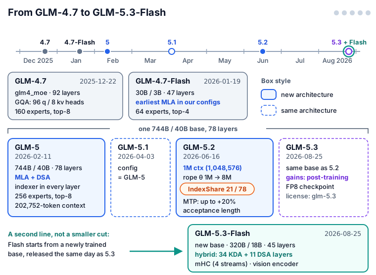
GLM-5.3 and GLM-5.3-Flash arrive at the end of a fast run of releases. This section places them on that timeline and then lines the two up in one table. The short version: one 744B skeleton carried GLM-5 through GLM-5.3, while Flash is a new design.

1.1 From GLM-4.7 to GLM-5.3-Flash

The animation below traces the lineage through the configs. Dates are the Hugging Face repository creation dates.

GLM-5 through GLM-5.3 share one 744B / 40B skeleton: the architecture changed at GLM-5 (MLA + DSA) and at GLM-5.2 (1M context, IndexShare), and GLM-5.3's gains come from post-training. GLM-5.3-Flash came out the same day, but it is a separate, newly trained hybrid base, not a smaller cut of GLM-5.3. Open the full-size SVG.

Model	Date	model_type	Total / active	Layers	Attention	Routed experts (top-k)	Context
GLM-4.7	2025-12-22	glm4_moe	not stated	92	grouped-query attention (GQA), 96 query / 8 KV heads	160 (top-8)	202,752
GLM-4.7-Flash	2026-01-19	glm4_moe_lite	30B / 3B	47	MLA	64 (top-4)	202,752
GLM-5	2026-02-11	glm_moe_dsa	744B / 40B	78 + 1 MTP	MLA + DSA, indexer on every layer	256 (top-8)	202,752
GLM-5.1	2026-04-03	glm_moe_dsa	744B / 40B	78 + 1 MTP	same config as GLM-5	256 (top-8)	202,752
GLM-5.2	2026-06-16	glm_moe_dsa	744B / 40B	78 + 1 MTP	MLA + DSA with IndexShare (21 of 78 layers run an indexer)	256 (top-8)	1,048,576
GLM-5.3	2026-08-25	glm_moe_dsa	same base as GLM-5.2	78 + 1 MTP	same config as GLM-5.2	256 (top-8)	1,048,576
GLM-5.3-Flash	2026-08-25	glm5_next	320B / 18B	45 + 1 MTP	34 KDA + 11 DSA (hybrid)	288 (top-8)	1,048,576

Every model in the table also has one shared expert that sees every token. Read top to bottom, the table shows three real architecture jumps and several releases that kept the same shape:

• GLM-4.7 → GLM-5. GQA, where 8 key/value heads serve 96 query heads, gives way to MLA plus DSA, in a shallower model with more experts. GLM-4.7-Flash, a 30B model, is the earliest MLA model among the configs we read.
• GLM-5 → GLM-5.1. Nothing structural. The two configs differ only in the transformers_version field.
• GLM-5.1 → GLM-5.2. A 1M-token window with a larger rotary base (§6), IndexShare (§5.6), an fp32 router (§4), and, per the GLM-5.2 card, an improved MTP layer whose acceptance length is “up to 20%” higher.
• GLM-5.2 → GLM-5.3. Same architecture again, now packaged in FP8 (§6.3); the card credits post-training for every gain.
• GLM-5.3-Flash. A new branch: a newly trained 320B base model with a hybrid of linear and sparse attention, mHC residual streams, and a vision encoder. It is the first natively multimodal model in the GLM-5 series, according to its card.

Licenses changed too. GLM-5.2 and GLM-5.3-Flash are MIT-licensed. GLM-5.3’s card lists license: other with the name glm-5.3; its terms are not part of the sources we read.

Where the numbers come from

• Layer counts, attention types, expert counts, and context lengths come from each model’s config.json (num_hidden_layers, num_nextn_predict_layers, n_routed_experts, num_experts_per_tok, max_position_embeddings).
• GLM-5’s 744B / 40B comes from the GLM-5 report and the Miles model index; GLM-5.1 and GLM-5.2 carry the same figure in the Miles docs. GLM-4.7-Flash’s 30B / 3B comes from the Miles docs. GLM-5.3-Flash’s 320B / 18B comes from its model card. GLM-4.7’s size is not stated in the sources we read.
• The GLM-5.3 card gives no parameter count. Since it shares GLM-5.2’s base model, it inherits GLM-5.2’s 744B / 40B; that is an inference from the card, not a number on it.
• The GLM-5 report says the model has 80 layers; every config from GLM-5 to GLM-5.3 says 78 decoder layers plus 1 MTP layer. We follow the configs.
• The config key head_dim changes from 64 to 192 in GLM-5.2, while the MLA dimensions it might describe stay the same. We treat it as metadata.

1.2 GLM-5.3 and GLM-5.3-Flash Side by Side

The two new models share a vocabulary, a context length, an indexer shape, and a routing scheme. Almost everything else differs:

	GLM-5.3	GLM-5.3-Flash
Base model	same as GLM-5.2	newly trained
Total / active parameters	744B / 40B (inherited from GLM-5.2’s base; official figure from the GLM-5 report)	320B / 18B (model card)
Decoder layers	78 (+1 MTP)	45 (+1 MTP)
Hidden size	6,144	4,096
Attention layers	78 × MLA + DSA	34 × KDA + 11 × MLA + DSA, as [KDA, KDA, KDA, DSA] × 11 + one KDA
MLA query / KV ranks	2,048 / 512	1,536 / 512
Query/key head dimensions	256 = 192 without position + 64 with RoPE	256, all without position
Position encoding	RoPE, rope_theta 8,000,000	none (NoPE)
Indexer layers	21 compute, 57 reuse (IndexShare)	11, each scoring one pooled key per 4 tokens
Indexer heads × dim / keys kept	32 × 128 / 2,048	32 × 128 / 2,048
Feed-forward layers	3 dense (0–2) + 75 MoE	3 dense (0–2) + 42 MoE
Experts per MoE layer	256 routed + 1 shared, top-8	288 routed + 1 shared, top-8
Residual stream	one standard stream	mHC, 4 streams
Vision	none (text only)	24-layer vision transformer (ViT)
License	other (glm-5.3)	MIT

Two terms in the table need a word now; later sections explain them fully. RoPE (rotary position embedding) tells attention where each token sits by rotating part of each query and key vector. NoPE means no position embedding at all. “Compute” and “reuse” indexer layers are the IndexShare split: a compute layer picks its own 2,048 tokens, and a reuse layer copies the pick of the nearest earlier compute layer.

Where the numbers come from

• Every structural row comes from the two config.json files. For Flash the keys live under text_config and vision_config; the layer mix is layer_types (34 linear_attention, 11 deepseek_sparse_attention), and the NoPE row is qk_rope_head_dim: 0 with mla_use_nope: true and no rope_theta.
• The indexer rows: GLM-5.3’s indexer_types lists 21 full and 57 shared layers; Flash’s lists all 45 as full and adds index_kpool: 4. Only Flash’s 11 DSA layers have an attention indexer.
• Both checkpoints’ configs carry an FP8 (e4m3, 128 × 128 block) quantization_config.
• The parameter row quotes published figures (GLM-5 report, Miles docs, Flash card). Our own recounts from the configs land close to them but follow different counting conventions; §2 and §8 show the arithmetic.

1.3 Two Stories

The rest of the post follows a simple split. GLM-5.3 is a training story: its architecture is GLM-5.2’s, so §2–6 explain that inherited 744B design, and §7 asks where the new model’s gains came from. GLM-5.3-Flash is an architecture story: §8 takes apart its new hybrid, and §9 compares what each design costs at long context.

The two stories meet in one place. Both models run an indexer on about one layer in four, by different routes. GLM-5.3 gets there by sharing (21 of 78 layers, 26.9% by our count), and Flash by its layout (11 of 45 layers, 24.4%).

2. A Tour of GLM-5.3’s 78 Layers

What happens to one token on its way through GLM-5.3? It passes through 78 layers that all share one shape: an attention block, then a feed-forward block. The layers differ in only two ways, and this section shows where.

2.1 The Path of a Token

1. Embedding. The token’s ID selects one row of a 154,880 × 6,144 table. From here on the token is a vector of 6,144 numbers, the hidden state.
2. Layers 0–2. Each layer runs MLA attention with DSA token selection, then a dense SwiGLU feed-forward network (FFN; a gated MLP) whose inner width is 12,288.
3. Layers 3–77. The same attention, but the feed-forward block is an MoE layer: 256 routed experts plus 1 shared expert, and each token visits 8 routed experts plus the shared one.
4. Output. A final normalization, then an output projection (lm_head) from 6,144 numbers to 154,880 vocabulary scores. The projection is untied: it does not reuse the embedding table.
5. MTP layer (index 78). One extra full decoder layer drafts a further token for speculative decoding (a cheap draft that the full model then checks in one pass). §6 covers it.

Every one of the 78 layers uses the same attention design. MLA compresses what each token stores for later attention into a small latent vector (§3). DSA then lets each query read at most 2,048 past tokens, picked by a cheap scorer called the lightning indexer (§5).

Implementation notes

• The dense/MoE split is the config’s mlp_layer_types (3 dense, 75 sparse), consistent with first_k_dense_replace: 3. tie_word_embeddings is false.
• The MTP layer is model.layers.78 in the module names listed in the FP8 config. It has its own attention, indexer, and MoE router, plus modules named eh_proj, enorm, hnorm, and shared_head.norm. Our reading, following the DeepSeek-V3-style layout these names point to: eh_proj maps the concatenation of a normalized embedding and a normalized hidden state (2 × 6,144) back to 6,144, and the layer shares the main model’s embedding and lm_head.

2.2 Which Layers Run an Indexer

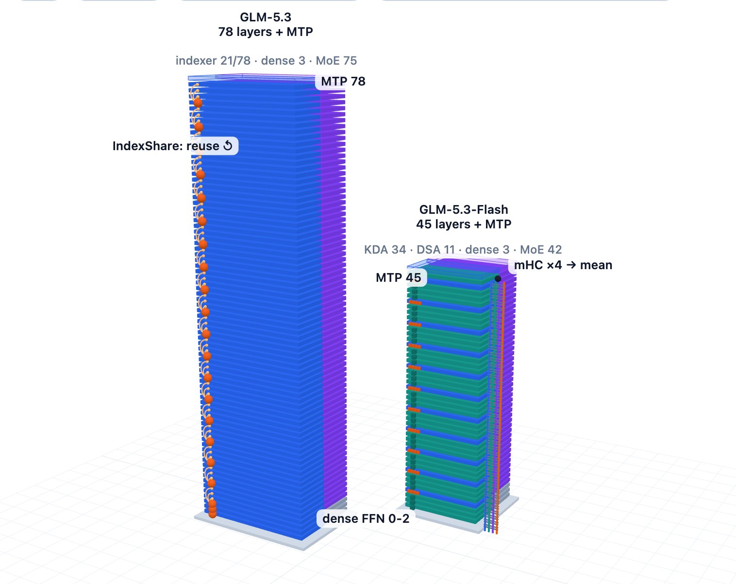
The first variation is the feed-forward block: dense in layers 0–2, MoE everywhere else. The second is the indexer. In GLM-5 and GLM-5.1, every layer ran its own. Since GLM-5.2, only 21 of the 78 layers do:

\[0,\ 1,\ 2,\ 6,\ 10,\ 14,\ \dots,\ 70,\ 74\]

The other 57 layers reuse the selection of the nearest earlier indexer layer. After the first two layers, the pattern settles into groups of four: one layer that computes, then three that reuse.

\[\{0\},\ \{1\},\ \{2 \mid 3, 4, 5\},\ \{6 \mid 7, 8, 9\},\ \dots,\ \{74 \mid 75, 76, 77\}\]

The config encodes this with two numbers, an offset of 3 and a frequency of 4. In the 0-indexed numbering used above, layer $\ell$ runs its own indexer exactly when

\[\ell \le 2 \quad\text{or}\quad (\ell - 2) \bmod 4 = 0 .\]

So layer 6 computes ($6 - 2 = 4$), while layer 3 does not and reuses the tokens that layer 2 picked. That makes 2 standalone layers plus 19 groups of four, or 21 indexer layers, so 73.1% of the indexer passes (57 of 78) disappear. §5 explains why neighboring layers can share a selection at all.

Implementation notes

• The config keys are index_skip_topk_offset: 3 and index_topk_freq: 4, and the explicit 78-entry list indexer_types (21 full, 57 shared). We checked that the formula above reproduces that list exactly. In the config’s own 1-indexed form ($L = \ell + 1$), the rule reads $\max(L - 3,\ 0) \bmod 4 = 0$.
• The same rule appears in Miles as is_skip_topk_layer (miles_plugins/models/glm5/glm5.py), with a comment that it mirrors _get_skip_topk_flags in glm-train-prod. A helper, source_compute_layer, returns the layer whose selection a shared layer reuses.
• Miles’ GLM-5.2 docs list the computing layers in 1-indexed form: 1, 2, 3, 7, 11, …, 75.
• One coincidence stands out. The first three layers are both the dense layers and the three leading indexer layers, and both rules use an offset of 3. Our reading is that this is a convenient alignment; the config sets the two independently (first_k_dense_replace and index_skip_topk_offset), and no source says they are coupled.

In the 3D model below, switch to GLM-5.3 alone to follow the indexer pattern, or tap a layer for its type and derived parameter count.

GLM-5.3 (78 layers + MTP) stands next to GLM-5.3-Flash (45 + MTP) at equal layer spacing, while a token climbs each tower: only 21 GLM-5.3 layers run an indexer and the rest reuse its pick, while Flash interleaves 34 KDA layers with 11 DSA layers inside four mHC streams. Drag to rotate, hover or tap any layer for its details, and use the toggles to show one model or to highlight the indexer, attention, FFN or mHC (layer types and counts come from the configs; per-layer parameter counts are derived and the token path is schematic).

2.3 Where the Parameters Live

Nearly all of GLM-5.3’s weights sit in the routed experts, and any one token uses only a few of them. The breakdown below is derived from the config; the official figures (GLM-5 report) are 744B total and 40B active.

Component (derived from the config)	Parameters	Share of 753.3B
Routed experts (75 layers × 256 × 37.75M)	724.8B	96.2%
MLA attention (78 layers × 165.0M)	12.9B	1.7%
MTP layer	9.95B	1.3%
Shared experts (75 × 37.75M)	2.83B	0.4%
Embedding table + lm_head	1.90B	0.3%
Dense feed-forward (3 × 226.5M)	0.68B	0.09%
Lightning indexers (21 × 9.37M)	0.197B	0.03%
Routers (75 layers)	0.118B	0.02%
Everything, by our count	753.3B

Attention and indexers together are under 2% of the model. The indexer, which §5 shows can dominate long-context prefill time (prefill is the pass that processes the whole prompt at once), is 0.03% of the weights.

The active count tells the other half of the story. In each MoE layer a token touches 8 of 256 routed experts plus the shared one. Counted the way the GLM-5 report counts (MTP included, embedding table and lm_head excluded), we get 39.94B active parameters per token, which matches the official 40B.

Why 744B and not 753B?

The GLM-5 report (Table 10) gives 744B total and 40B active, and says it counts the MTP layer but not the word embeddings or the output layer. Our recount depends on that choice:

Convention (derived)	Total	Active
Every module we count	753.3B	41.84B
GLM-5 report: MTP in, embeddings and lm_head out	751.4B	39.94B
Embeddings and lm_head in, MTP out	743.4B	41.25B

Under the report’s own convention the active count matches, but our total lands about 1% above 744B; the closest total comes from dropping MTP instead. Either our assumed shapes differ slightly from the checkpoint, or the published total follows a different convention than stated. We cannot settle this without the checkpoint’s tensor index, so we quote the official 744B / 40B and treat our numbers as a recount within about 1%.

Our assumptions: DeepSeek-V3/V3.2 module shapes for MLA and the MoE layers; indexer shapes as in Miles (wq_b, wk, a LayerNorm, weights_proj); indexer weights only on the 21 computing layers and the MTP layer; shared experts the same size as routed experts; no biases except the router’s expert bias. Norms (about 1M parameters in total) are left out of the table above but included in the totals.

3. MLA: Caching a 576-Number Summary Instead of Full Keys and Values

To write the next token, an attention layer can look back at any earlier token, so the model keeps a key-value (KV) cache for every token, and at long context that cache is what fills GPU memory. MLA, introduced in the DeepSeek-V2 paper, keeps one short compressed vector per token per layer and rebuilds each head’s keys and values from it on demand. In GLM-5.3 that vector holds 576 numbers.

3.1 The problem: a cache that grows with every token

Attention works like a lookup. The newest token forms a query, compares it with a key from every earlier token, and mixes those tokens’ values according to the scores. Keys and values of past tokens never change, so instead of recomputing them at every step the model stores them. That store is the KV cache: one entry per token per layer, kept for the whole conversation, and read again every time a token is generated.

How big is one entry? It depends on the attention design:

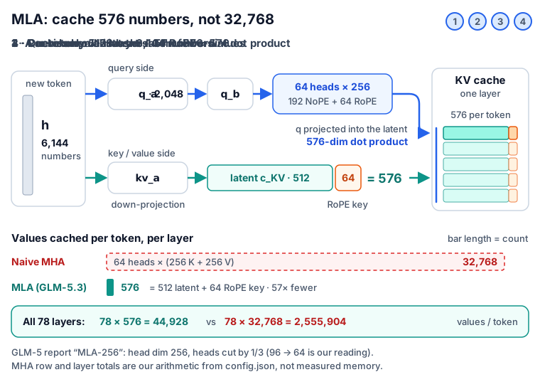
• Multi-head attention (MHA) caches a full key and a full value for every head. The DeepSeek-V2 paper writes this as $2 n_h d_h$ values per token per layer ($n_h$ heads of size $d_h$). With GLM-5.3’s head sizes, 64 heads with 256-dimension keys and 256-dimension values, that is 64 × (256 + 256) = 32,768 values.
• GQA lets several query heads share one key/value head. GQA-8, the baseline in the GLM-5 report, has 8 key/value heads of 128 dimensions (2 × 8 × 128 = 2,048), a “2048-dimension KV-cache”.
• MLA caches one 512-number latent plus one 64-number position key, 576 values, shared by all 64 heads.

Cache design (per token, per layer)	Values cached	Share of naive MHA (derived)	Where the number comes from
Naive MHA: 64 heads × (256 K + 256 V)	32,768	100%	derived from GLM-5.3’s dimensions
GQA-8 (the GLM-5 report’s baseline)	2,048	6.25%	GLM-5 report
MLA in GLM-5.3: 512 latent + 64 RoPE key	576	1.76%	config; the report calls it a “576-dimension latent KV-cache”

Stacked over 78 layers, MLA caches 78 × 576 = 44,928 values per token, about 88 KiB in bf16, a 16-bit format with 2 bytes per value (derived from the config). The naive design would need 78 × 32,768 = 2,555,904 values, roughly 57 times more (derived). §9 turns these per-token figures into totals at a million tokens.

A smaller cache is only useful if quality survives. The DeepSeek-V2 paper’s ablation is the main evidence: at two MoE scales, MLA kept 14% and 4% of MHA’s cache and still scored higher on most of the reported benchmarks. The rest of this section shows how 576 numbers can stand in for 32,768.

Where the numbers come from

• DeepSeek-V2 Table 1 gives the per-token cache as $2n_hd_hl$ for MHA, $2n_gd_hl$ for GQA with $n_g$ groups, and $(d_c+d_h^R)\,l$ for MLA ($l$ layers). DeepSeek-V2 itself used $d_c = 512$ and $d_h^R = 64$, the same 576 as GLM-5.3, which the paper equates to “GQA with only 2.25 groups” at its head size of 128.
• DeepSeek-V2 Table 9 (ablation): KV cache per token 110.6K (MHA) vs 15.6K (MLA) for the small MoE model and 860.2K vs 34.6K for the large one. MLA scores higher on BBH, MMLU, and CMMLU at both scales; on C-Eval the small MLA model is slightly lower (50.9 vs 51.6).
• GLM-5.3 numbers use the config keys num_attention_heads 64, qk_head_dim 256, v_head_dim 256, kv_lora_rank 512, qk_rope_head_dim 64, and num_hidden_layers 78. Byte counts assume 2 bytes per value; the sources do not say how deployments store the cache (it may be FP8), and the DSA indexer’s own key cache (§5) is not included.

3.2 Compression: one latent per token, re-expanded per head

MLA replaces “store every head’s key and value” with “store a short summary, and derive keys and values from it”. Here are the shapes involved; matrices are written as [output × input].

\(h_t\in\mathbb{R}^{6144}\)Hidden state of token \(t\) entering the attention block.

\(c_t\in\mathbb{R}^{512}\)The KV latent (kv_lora_rank), made by \(W^{DKV}\) [512 × 6,144] plus an RMSNorm. Cached.

\(k^R_t\in\mathbb{R}^{64}\)The RoPE key (qk_rope_head_dim), made by \(W^{KR}\) [64 × 6,144], shared by all heads. Cached (§3.3).

\(W^{UK}_i\), \(W^{UV}_i\)Per-head up-projections, [192 × 512] for the key and [256 × 512] for the value, for heads \(i = 1,\dots,64\).

\(c^Q_t\in\mathbb{R}^{2048}\)The query latent (q_lora_rank), covered in §3.5.

When token $t$ passes through a layer, three things happen:

1. Down-project. The 6,144-wide hidden state is squeezed to 512 numbers and normalized: $c_t=\mathrm{RMSNorm}(W^{DKV}h_t)$. This latent carries no position information.
2. Cache. The latent goes into the cache together with the 64-number RoPE key $k^R_t$, computed from $h_t$ as $k^R_t=\mathrm{RoPE}(W^{KR}h_t)$. That pair, 576 numbers, is all the layer stores for this token.
3. Re-expand when needed. Each head $i$ recovers its own 192-number content key and 256-number value from the shared latent, and appends the shared RoPE key to the key (this is the training/prefill view; §3.4 shows decoding skips the expansion):

\[k_{t,i}=\big[\,\underbrace{W^{UK}_i c_t}_{192}\,;\;\underbrace{k^R_t}_{64}\,\big]\in\mathbb{R}^{256}, \qquad v_{t,i}=W^{UV}_i c_t\in\mathbb{R}^{256}\]

In plain terms: instead of writing 64 separate key-value pairs for each token, the layer writes one 576-number note that each of the 64 heads reads through its own lens.

A toy version makes the trade concrete. Suppose the latent has 2 numbers, $c=(1,2)$, and head 1’s key matrix has rows $(1,0)$, $(0,1)$, $(1,1)$; its key is $(1,2,3)$. Head 2’s matrix has rows $(2,0)$, $(0,0)$, $(1,-1)$, so its key is $(2,0,-1)$. Six key numbers come out, but only two were stored. The price is that the heads’ keys cannot vary independently: all 64 × 192 = 12,288 content-key numbers are linear functions of the same 512. MLA bets that 512 directions are enough, which is what DeepSeek-V2’s ablation tested.

Per token and per layer, GLM-5.3's MLA caches only a 512-number latent plus a 64-number RoPE key (576 values); queries are projected into that latent so attention reads the cache directly. The naive-MHA comparison (32,768) and the 78-layer totals are our arithmetic from config.json, not measured memory. Open the full-size SVG.

Implementation notes

• In Miles (the open training framework whose GLM-5 code we read; §10), $W^{DKV}$ and $W^{KR}$ are one fused matrix, linear_kv_down_proj, of shape [576 × 6,144], split after the matmul into the 512-number latent and the 64-number RoPE key (glm5/glm5.py). Following DeepSeek-V2’s equation 15, the RoPE key is computed from $h_t$, not from the latent.
• All 64 heads’ $W^{UK}_i$ and $W^{UV}_i$ live in one matrix, linear_kv_up_proj, of shape [64 × (192 + 256) = 28,672 × 512], whose RMSNorm weight normalizes the latent.
• Naming trap: in Megatron and Miles, qk_head_dim means the 192-dimension NoPE part and qk_pos_emb_head_dim the 64-dimension RoPE part. In the Hugging Face config the same numbers are qk_nope_head_dim 192 and qk_rope_head_dim 64, and qk_head_dim is their sum, 256.

3.3 Decoupled RoPE: position gets its own small channel

Attention also needs to know where tokens are. RoPE supplies this by rotating pairs of query and key dimensions through an angle proportional to the token’s position. When a query at position $t$ meets a key at position $j$, the two rotations combine into one rotation by the distance $j-t$, so the score depends on how far apart the tokens are.

That is exactly what clashes with MLA. The decode trick in §3.4 relies on moving $W^{UK}_i$ over to the query side. If RoPE were applied to the re-expanded key $W^{UK}_i c_j$, a rotation that depends on the two tokens’ positions would sit between the query and $W^{UK}_i$. Every cached token would need a different combined matrix, and the folding no longer works. The DeepSeek-V2 paper puts the consequence bluntly: “we must recompute the keys for all the prefix tokens during inference.”

MLA’s fix, which the paper calls decoupled RoPE, keeps the two jobs apart:

• Content lives in the 192-number part of each head’s query and key. It never rotates, so it can be folded.
• Position lives in a separate 64-number part: each head gets its own rotated query slice $q^R_{t,i}$, while the key side has one rotated key $k^R_t$ shared by all 64 heads. Because $k^R_t$ comes straight from $h_t$ and is cached already rotated, nothing ever needs folding through it.

Each head’s full query and key are 256 numbers, 192 NoPE (no position) plus 64 RoPE:

\[q_{t,i}=\big[\,q^C_{t,i}\,;\;q^R_{t,i}\,\big],\qquad k_{j,i}=\big[\,W^{UK}_i c_j\,;\;k^R_j\,\big],\qquad \mathrm{score}_i(t,j)=\frac{q^C_{t,i}\cdot W^{UK}_i c_j\;+\;q^R_{t,i}\cdot k^R_j}{\sqrt{256}}\]

Here $q^C_{t,i}$ (192 numbers) and $q^R_{t,i}$ (64) are head $i$’s content and rotated query parts, built from the query latent in §3.5.

In plain terms: the score is a content match plus a position-aware match, added together, and only the small second term involves rotation. The cost is the 64 extra numbers per token in the cache, which is why the entry is 576 and not 512.

GLM-5.3’s rope_theta of 8,000,000 (up from 1,000,000) arrived with GLM-5.2’s 1M context; rope_interleave true and the missing scaling entry date back to GLM-5. §6 covers them.

Why the rotation blocks folding, in one line

Write the rotation at position $p$ as an orthogonal matrix $R_p$. With RoPE on the full key, the content score would be $(R_t q)^\top (R_j W^{UK}i c_j) = q^\top R{j-t}\, W^{UK}i c_j$. The matrix $R{j-t}$ changes with every cached position $j$, and matrix products do not commute, so $W^{UK}i$ cannot be merged into one fixed per-head query matrix. With decoupled RoPE the rotation touches only $q^R{t,i}$ and $k^R_j$, and the content term $q^{C\top}_{t,i} W^{UK}_i c_j$ has nothing in the middle. The DeepSeek-V2 paper gives the argument in words (Section 2.1.3); the formula is our restatement.

Fine print: Miles applies RoPE in the interleaved layout (rope_interleave true), and its softmax scale is $1/\sqrt{256}$ times the square of a YaRN mscale factor computed from the run’s rotary-scaling settings; DeepSeek-V2’s equation 18 uses $1/\sqrt{d_h+d_h^R}$.

3.4 The decode trick: absorb the up-projections

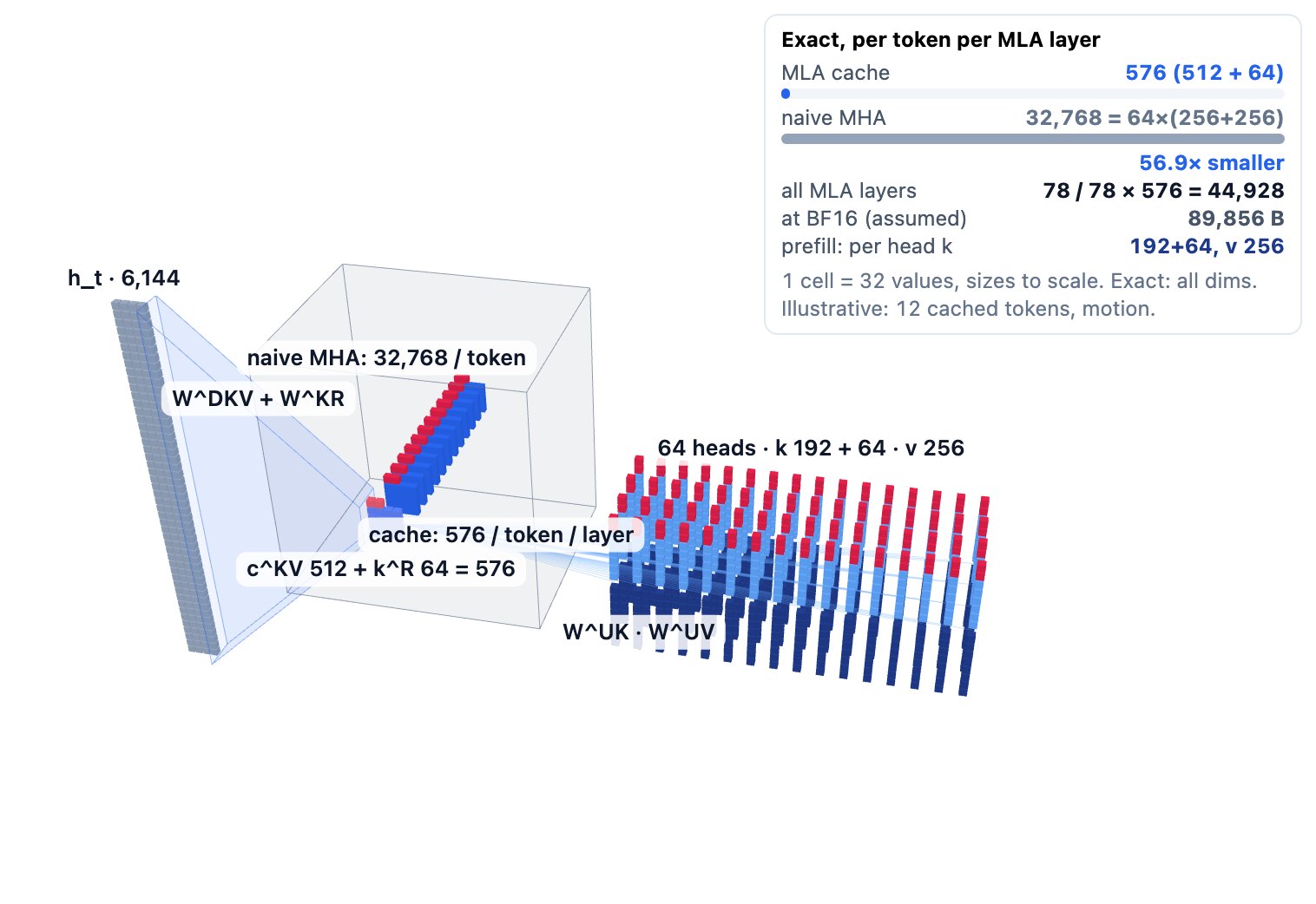
Re-expanding every cached latent into 64 keys and values at every decoding step would throw away the savings: the cache would be small, but each step would redo the expansion for the whole prefix. MLA avoids this with a rewrite that the DeepSeek-V2 paper calls absorbing $W^{UK}$ into the query and $W^{UV}$ into the output. It is just associativity of matrix products:

\[\mathrm{score}_i(t,j)\cdot\sqrt{256}=q^{C}_{t,i}\cdot\left(W^{UK}_i c_j\right)+q^{R}_{t,i}\cdot k^R_j =\underbrace{\left(W^{UK\top}_i q^{C}_{t,i}\right)}_{512\text{ numbers}}\cdot\,c_j+\underbrace{q^{R}_{t,i}}_{64}\cdot\,k^R_j\]

For one new token, each head then does four things:

1. Translate the query once. Multiply the 192-number content query by $W^{UK\top}_i$ to get a 512-number query in “latent language”. Glue the 64-number RoPE query on: 576 numbers.
2. Score every cached entry directly. Each score is one 576-number dot product against the cached $[c_j; k^R_j]$. The cache entry is identical for all 64 heads.
3. Mix latents, not values. The softmax-weighted sum runs over the cached 512-number latents $c_j$, which double as values.
4. Expand once at the end. Apply $W^{UV}_i$ [256 × 512] to that single sum, then the output projection.

In plain terms: the expansion happens once per new token instead of once per cached token. The GLM-5 report states the resulting cost directly: “MLA performs a 576-dimensional dot product, higher than the 128-dimensional computation of GQA.”

Why trade more arithmetic for fewer bytes? Decoding produces one token per sequence per step, so typically most of the time goes to reading the cache from GPU memory, and the arithmetic units wait on it. By our count, in floating-point operations (FLOPs) per attended token and per layer:

Decode attention, one new token (derived)	FLOPs	Bytes read (bf16)	FLOPs per byte
Naive MHA: 64 heads × (256 K + 256 V)	65,536	65,536	1.0
Absorbed MLA: 64 heads × (576 score + 512 mix)	139,264	1,152	about 121

MLA does about 2.1 times the arithmetic and reads about 57 times fewer bytes. Under DSA each query attends to at most 2,048 tokens (§5), so the MLA part of one layer reads about 2.4 MB of cache per new token, where naive MHA would read 134 MB for the same 2,048 tokens (by our count). On layers that run the indexer, its scan of every earlier token’s index key comes on top (§5.3). Without absorption, re-expanding those 2,048 latents through the [28,672 × 512] up-projection would cost about 60 GFLOPs per layer per token, against about 0.29 GFLOPs for the absorbed core.

The 3D model below shows both paths, the expanded form used in training and prefill and the absorbed form used in decoding; its Flash mode returns in §8.4.

MLA squeezes each token's 6,144-d hidden state into one 512-d latent plus a 64-d RoPE key, so the cache grows by just 576 values per token per layer instead of the 32,768 naive 64-head attention would need (56.9× less; Flash caches 512 with no RoPE, 64× less). Prefill expands the latent back into 64 heads; decode absorbs W^UK into the query (192 → 512) and W^UV into the output (512 → 256), so attention runs directly on the cached latents.

Assumptions and code-level notes

• Cost model (ours): FLOPs = 2 × multiply-adds; softmax, RoPE, and norms ignored; 2 bytes per cached value; weight reads ignored (they are shared across a batch). MLA per attended token: $2\cdot64\cdot576 + 2\cdot64\cdot512 = 139{,}264$ FLOPs and $576\cdot2 = 1{,}152$ bytes. At 131,072 attended tokens (dense attention) the same layer would read about 151 MB with MLA and 8.6 GB with naive MHA.
• No-absorption cost: $2\cdot512\cdot28{,}672 \approx 29.4$ MFLOPs per cached token per step, about 60.1 GFLOPs at 2,048 tokens.
• One could literally precompute $W^{UK\top}_i W^{UQ}_i$ per head, but at these sizes the two-step form is cheaper (about 62.9 vs 134.2 MFLOPs per token, by our count), because the 192-number NoPE query is smaller than the 512-number latent. The same holds for merging $W^{UV}_i$ into $W^O$. Miles keeps the two steps as einsum calls in glm5/glm5.py.
• Miles runs the absorbed form in training too: the query is [tokens × 64 × 576], the key [tokens × 576], fed to a sparse MLA kernel. The DeepSeek-V3.2 paper likewise implements DSA on “the MQA mode of MLA” (MQA: multi-query attention, §5.2), where each latent is shared across all query heads. Whether Z.ai trains GLM-5.3 this way is not stated.

3.5 The query path and the parameter count

Queries are compressed too, though for a different reason. The hidden state goes through a down-projection to 2,048 numbers (q_lora_rank), an RMSNorm, and an up-projection to 64 heads × 256 dimensions: 192 NoPE and 64 RoPE dimensions per head. Queries are never cached, so this saves no cache memory; the DeepSeek-V2 paper says it was done to reduce activation memory during training. §5 shows that the DSA indexer reads this same 2,048-wide query latent.

Putting the pieces together, one MLA block holds about 165.0M parameters by our count:

Matrix	Shape [out × in]	Parameters (derived)
$W^{DQ}$, query down-projection	2,048 × 6,144	12.58M
$W^{UQ}$ + $W^{QR}$, query up-projection (fused)	64 × 256 = 16,384 × 2,048	33.55M
$W^{DKV}$ + $W^{KR}$, latent + RoPE key (fused)	576 × 6,144	3.54M
$W^{UK}$ + $W^{UV}$, all heads (fused)	64 × (192 + 256) = 28,672 × 512	14.68M
$W^O$, output projection	6,144 × 16,384	100.66M
Total per layer		165.02M

Across 78 layers that is about 12.9B, under 2% of the model (§2.3). Most of it is the output projection. The matrices that write and read the cache are small: the down-projection that produces each 576-number entry has only 3.54M parameters. Running all five matrices for one token costs about 330 MFLOPs per layer, twice the parameter count, regardless of context length.

Where the numbers come from

• Config keys (identical in GLM-5, 5.1, 5.2, and 5.3): num_attention_heads 64, num_key_value_heads 64, q_lora_rank 2048, kv_lora_rank 512, qk_nope_head_dim 192, qk_rope_head_dim 64 (so qk_head_dim 256), v_head_dim 256, attention_bias false. The GLM-5 report’s Table 10 lists Q LoRA Dim 2048 and KV LoRA Dim 512 for GLM-5.
• The shapes assume DeepSeek-V3-style projections with no biases and match Miles’ module definitions; norm weights (a few thousand values) are left out. These are our counts, not official figures.
• The two RMSNorms sit on the latents ($c^Q_t$ and $c_t$), following DeepSeek-V2, which adds normalization after the compressed latent vectors.

3.6 GLM-5’s adjustments: Muon Split and MLA-256

MLA’s small cache had a cost at first. GLM-5 was trained with the Muon optimizer, which orthogonalizes the update of each weight matrix, and with plain MLA the GLM-5 report found that a 576-dimension latent cache “cannot match the performance” of GQA-8 with its 2,048-dimension cache. The report describes two adjustments (no GLM-5.3 document discusses either). MLA-256 is visible in GLM-5.3’s config. Muon Split is a pre-training optimizer recipe, and no source says whether the GLM-5.2 base that GLM-5.3 builds on was trained with it.

Muon Split orthogonalizes the up-projections $W^{UQ}$, $W^{UK}$, and $W^{UV}$ per head instead of as whole matrices, so each head’s weights can update at their own scale. The report summarizes the result as Muon Split letting MLA “match” GQA-8. Its Table 1 is mixed in detail: Split wins on MMLU and C-Eval (and narrowly on Hellaswag and RACE, not shown below) and still trails on BBH, GSM8K, and HumanEval. The report adds a side effect: with Muon Split, GLM-5’s attention-logit scale “remains stable during pre-training without any clipping strategy.”

A selection from the report's Table 1

Variant	MMLU	C-Eval	BBH	GSM8K	HumanEval
GQA-8	61.2	60.0	53.3	47.6	38.5
MLA	61.5	59.7	48.9	46.2	33.5
MLA + Muon Split	62.5	62.1	51.8	45.0	36.7
MLA-256 + Muon Split	62.0	59.9	51.3	47.5	36.6

MLA-256 targets the decode arithmetic from §3.4. The report notes that DeepSeek-V3 chose its head count for the H800’s roofline, a choice that does not suit other hardware. GLM-5 therefore increases the head dimension “from 192 to 256” and decreases the number of attention heads “by 1/3”, which “keeps the training computation and the number of parameters constant while decreasing the decoding computation.” The last row of Table 1 shows it holding roughly level with MLA + Muon Split.

Why fewer heads help decoding, by our reading: in the absorbed form each head pays $576 + 512$ multiply-adds per cached token whatever its head dimension, so decode attention cost is $2 \cdot n_h \cdot 1{,}088$ FLOPs per attended token and scales with the head count $n_h$ alone. The report describes MLA as “MHA style” during training and prefilling, and in that expanded form wider heads make up for fewer heads. For illustration, a hypothetical 96-head version of GLM-5.3 would cost 208,896 FLOPs per cached token instead of 139,264.

Where the numbers come from

• The report’s Table 10 lists “QK Head Dim 192” for GLM-5, which matches qk_nope_head_dim; the config’s full query/key head is 192 + 64 = 256. Our reading is that “from 192 to 256” refers to the full head (128 + 64, as in DeepSeek-V2, becoming 192 + 64), but the report does not spell this out.
• The report does not name the head count MLA-256 cut from. GLM-4.5 had 96 heads (report Table 10), and 96 × 2/3 = 64 matches GLM-5.3’s config, so by our reading the baseline was plausibly 96. Treat this as a guess.
• “MLA-256” is the report’s name; the GLM-5.3 config contains only the dimensions.

3.7 Where MLA shows up next

• DSA runs on top of MLA (§5). The lightning indexer picks at most 2,048 earlier tokens, and absorbed MLA from §3.4 then attends only to their 576-number entries. The indexer keeps its own small key cache on the layers that compute it.
• GLM-5.3-Flash uses a NoPE MLA (§8.3, §8.4). Keep the 192/64 split in mind: Flash takes it to the limit, with a rotated part zero dimensions wide. Its cache entry is the bare 512-number latent, and only 11 of its 45 layers keep one.

  4. MoE: 256 Experts, 8 at a Time

An MoE layer replaces one large feed-forward network with many small ones, the experts, and lets a router choose a few of them for each token. This is where almost all of GLM-5.3’s parameters live, yet any single token uses only a small slice of them.

4.1 The layer in numbers

GLM-5.3’s feed-forward blocks come in two kinds:

• Layers 0–2 (dense): an ordinary SwiGLU feed-forward network, 6,144 → 12,288 → 6,144, about 226.5M parameters each (derived from the config).
• Layers 3–77 (MoE, 75 layers): 256 routed experts plus 1 shared expert. Each expert is a small SwiGLU network, 6,144 → 2,048 → 6,144, with 3 × 6,144 × 2,048 ≈ 37.75M parameters (derived).

For each token, the router picks 8 routed experts and the shared expert always runs:

256 + 1experts per MoE layerrouted + always-on shared

8routed experts per tokentop-8 by router score

37.75Mparameters per expertderived: 3 × 6,144 × 2,048

3.5%of the layer's FFN weights used per tokenderived: 339.7M of ~9.70B

Two comparisons make the trade visible (both by our count). Per token, an MoE layer does more feed-forward work than a dense layer (339.7M vs 226.5M parameters touched), yet it stores about 43 times as many weights. Summed over all 75 MoE layers, the 9 active experts account for roughly 25.5B of the 40B active parameters the GLM-5 report gives for this architecture (our count: 39.9B).

4.2 How the router picks 8 of 256

The config names the router’s pieces (keys in the notes below): sigmoid scoring, the aux-loss-free noaux_tc top-k method with a per-expert bias, renormalized weights, a scaling factor of 2.5, and a float32 router. Read with the standard DeepSeek-V3 semantics for these keys (our reading; the router code itself lives in Megatron-LM and SGLang, which we did not inspect), one token’s trip goes like this:

1. Score. Each expert $i$ gets an independent score $s_i=\sigma(e_i^\top h)$ between 0 and 1, computed in fp32.
2. Select. A per-expert bias $b_i$ is added, and the 8 highest values of $s_i+b_i$ win. With n_group = topk_group = 1, all 256 experts compete in one pool, with no group-limited routing.
3. Weight. The bias is dropped again. The winners’ raw scores are renormalized to sum to 1 and multiplied by 2.5.
4. Combine. The layer adds the shared expert’s output to the weighted sum of the 8 routed experts.

\[\mathcal{T}=\operatorname{top8}_i\,(s_i+b_i),\qquad g_i=2.5\cdot\frac{s_i}{\sum_{j\in\mathcal{T}}s_j}\ \ (i\in\mathcal{T}),\qquad y=E_{\text{shared}}(h)+\sum_{i\in\mathcal{T}}g_i\,E_i(h)\]

In plain terms: the bias decides who gets the token, the raw score decides how much each winner contributes. Example: expert 41 scores 0.70 with bias −0.10, and expert 7 scores 0.62 with bias +0.05. Selection compares 0.60 with 0.67, so expert 7 takes the slot. If the 8 winners’ raw scores sum to 4.0, expert 7’s weight is 2.5 × 0.62 / 4.0 ≈ 0.39.

4.3 Balance without an auxiliary loss

An MoE model fails quietly if a few experts receive most tokens while the rest sit idle. Many MoE models add an auxiliary load-balancing loss to the training objective. The noaux_tc scheme leans on the selection bias instead: in the recipe from the DeepSeek-V3 technical report (background, not one of our GLM sources), an overloaded expert’s bias is nudged down and an underused expert’s bias is nudged up, so the load evens out without a second loss term. Z.ai’s own bias-update schedule is not in our sources.

GLM-5.3’s config lists no auxiliary-loss coefficient at all. The explicit moe_router_dtype: float32 key first appears in GLM-5.2’s config. Our reading of why precision matters here: top-8 choices hinge on small differences between 256 scores plus small bias corrections, which low precision could blur.

The 3D model below lets you send tokens through a router like this one. Its scores and load patterns are synthetic and illustrate the mechanism, not GLM-5.3’s real routing.

The expert city: a token reaches the router, which scores all 256 expert pillars (288 in Flash), picks the top 8 with a selection-only bias and adds the always-on shared expert, so it uses 9 × 37.75M = 339.7M of 9.70B FFN weights (3.5%). Step through the four beats, switch between GLM-5.3 and Flash, turn bias correction on or off to compare the simulated 512-token load, and hover or tap any pillar for its numbers (counts and sizes are exact; scores, bias and loads are synthetic).

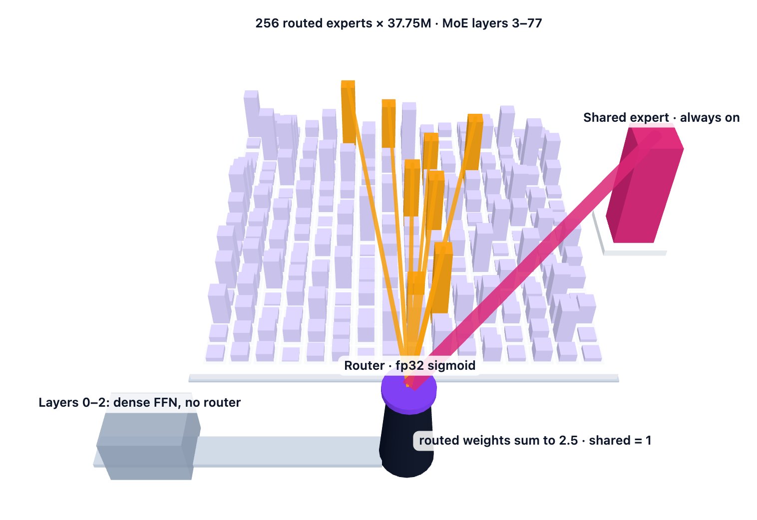
GLM-5.3-Flash keeps the same router recipe with 288 smaller experts and adds two new config keys; §8.7 covers the differences and revisits the 3D model in Flash mode.

Where the numbers come from

• Config keys (unchanged from GLM-5 through GLM-5.3): first_k_dense_replace 3, intermediate_size 12288, n_routed_experts 256, n_shared_experts 1, num_experts_per_tok 8, moe_intermediate_size 2048, scoring_func sigmoid, topk_method noaux_tc, norm_topk_prob true, routed_scaling_factor 2.5, n_group 1, topk_group 1. moe_router_dtype float32 is present from GLM-5.2 on. mlp_layer_types lists layers 0–2 as dense and 3–77 as sparse.
• The config does not state the shared expert’s width. We assume it equals moe_intermediate_size (2,048), the usual DeepSeek-V3 convention.
• 9.70B per MoE layer = 257 experts × 37.75M + a router of about 1.57M (256 × 6,144 weights + 256 biases). The model-wide split (routed experts ≈ 724.8B, over 96% of the total) is in §2.
• The MTP layer (layer 78) is also an MoE layer. In the FP8 checkpoint, the router weight (mlp.gate) and e_score_correction_bias stay unquantized on all 76 MoE layers (3–78).

Implementation notes: routing during reinforcement learning (RL) in Miles

• Miles’s GLM-5.3-Flash model script sets --moe-router-bias-update-rate 0, so the expert biases stay frozen during its RL runs; its GLM-5 and GLM-5.2 flagship scripts (glm5-744B-A40B.py, glm5.2-744B-A40B_lora.py) set the same flag. Its launcher can also turn on rollout routing replay (R3, --enable-r3 → --use-rollout-routing-replay), which makes training reuse the expert choices made at inference time; a code comment notes that “routing replay needs materialized topk ids.”
• The GLM-5 report brings up MoE routing replay only as an analogy when it explains why the DSA indexer’s top-k matters for RL stability (§5.7).
• These are choices in the open Miles implementation. They do not tell us how Z.ai trained GLM-5.3.

5. DeepSeek Sparse Attention and IndexShare: Read 2,048 Tokens, Choose Them Less Often

At a million tokens of context, letting every new token look at every earlier token is a fundamental bottleneck for a long-context model. GLM-5.3 avoids it in two steps. First, a cheap scorer picks the 2,048 earlier tokens that matter most, and the expensive attention reads only those. Second, because neighboring layers keep picking nearly the same tokens, most layers simply reuse an earlier layer’s picks.

5.1 Why sparse attention, and DSA’s two parts

Dense attention does work in proportion to the context. A token at position $L$ compares its query with all $L$ cached entries, so the cost per new token grows linearly with $L$, and processing a whole sequence grows with $L^2$. In GLM-5.3’s absorbed MLA (§3.4), one head pays a 576-number dot product per cached token for the score and a 512-number weighted sum for the output. Across 64 heads that is 69,632 multiply-adds per cached token, per layer (derived).

At $L$ = 1,048,576 this comes to about 73 billion multiply-adds per new token in a single layer, before any of the model’s weights are applied (derived). The roughly 40B active parameters of the shared GLM-5 / GLM-5.2 base (GLM-5 report, Table 10) cost about 40 billion multiply-adds per token for the whole 78-layer model (one per weight, a rough derived figure). At a million tokens, one layer of dense attention would cost more than all of them combined.

The cheap fixes discard information. The GLM-5 report (arXiv 2602.15763) tested two of them on GLM-9B, a 40-layer model, keeping half of the layers as full attention (1:1) and continuing training on 190B tokens at 64K:

• Sliding-window attention (SWA): each token sees only a fixed window of recent tokens.
• Linear attention: the growing KV cache is replaced with a fixed-size running memory (§8.2).

RULER (a long-context retrieval benchmark) at 128K, relative to full attention:

Variant (half the layers still full attention)	RULER@128K change
SWA Interleave (sliding window every other layer)	−30.35
SWA Pattern (searched placement of window layers)	−5.69
GDN (Gated DeltaNet, a linear-attention layer)	−11.28
SimpleGDN (the report’s lighter GDN variant)	−8.25

Every variant lost fine-grained retrieval accuracy even with half the layers left dense. The report concludes that DSA, unlike these, can run in every layer, and the flagship does exactly that: DSA in all 78 layers. Keep this table in mind for §8: GLM-5.3-Flash does adopt linear attention, but keeps a DSA layer in every group of four.

Where the numbers come from

• Cost per cached token: 64 heads × (576 + 512) = 69,632 multiply-adds, counting the absorbed-form score (512 latent + 64 RoPE dimensions) and the value sum over the 512-number latent, as in the Miles sparse kernel. Softmax, projections and the absorption matrices are ignored; they cost the same with or without sparsity. 69,632 × 1,048,576 ≈ 7.3 × 10¹⁰ is our arithmetic.
• Ablation (Table 5): GLM-5 report, Sec. 2.1.2. SWA = sliding-window attention (the report’s training-free Table 4 uses a 4,096-token window). These runs used GLM-9B, not GLM-5.

DSA’s idea. DSA keeps exact attention but makes it read less. It comes from DeepSeek-V3.2 (arXiv 2512.02556), where it is the only architectural change from DeepSeek-V3.1-Terminus, added by continued training. The paper describes two components:

1. A lightning indexer that gives every earlier token $s$ a relevance score $I_{t,s}$ for the current query token $t$, cheaply (§5.2).
2. Fine-grained token selection that keeps the $k$ highest-scoring tokens and runs the normal attention over only their cached MLA entries $c_s$ (§5.3).

In the V3.2 paper’s notation, the attention output $u_t$ is

\[u_t \;=\; \mathrm{Attn}\!\Big(h_t,\;\big\{\,c_s \;\big|\; I_{t,s}\in \mathrm{Top}\text{-}k\big(I_{t,:}\big)\big\}\Big)\]

In plain terms: a librarian first skims the whole catalog and pulls 2,048 books; the reader then studies only those. Skimming still touches every catalog card, so it must be far cheaper per card than reading. GLM-5.3 uses $k$ = 2,048 (index_topk), the same value as DeepSeek-V3.2. At a 1M-token context a layer then reads 2,048 of 1,048,576 tokens, about 0.2% (derived).

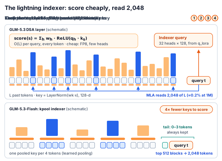
5.2 The lightning indexer in detail

The indexer is a miniature attention layer with one job: produce a single number per earlier token. For each query token $t$ it computes three things from that token’s own activations, and each earlier token $s$ contributes one thing:

Piece	Computed from	GLM-5.3 shape	Weights
Index queries $q_{t,1..32}$	MLA’s 2,048-wide compressed query (q_lora, §3.5), RMS-normalized, then projected	32 heads × 128	wq_b: 2,048 → 4,096
Head weights $w_{t,1..32}$	the token’s 6,144-wide hidden state	32 scalars	weights_proj: 6,144 → 32
Index key $k_s$	earlier token’s hidden state, projected, then a LayerNorm	one vector of 128	wk: 6,144 → 128, plus k_norm

The score of earlier token $s$ for query token $t$ is

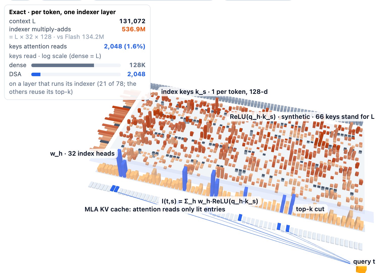
\[I_{t,s} \;=\; \sum_{j=1}^{32} w_{t,j}\;\mathrm{ReLU}\!\left(\mathbf{q}_{t,j}\cdot\mathbf{k}_{s}\right)\]

In plain terms: each of the 32 heads $j$ takes a 128-number dot product between its query and the token’s key, negative results are clipped to zero, and the heads are mixed with per-query weights. Do that for every earlier token, sort, keep the best 2,048.

A tiny example. Shrink the indexer to 2 heads and score two earlier tokens, A and B (made-up numbers):

	head 1 dot product	head 2 dot product	after ReLU	score with $w_t$ = (1.0, 0.5)
token A	0.8	−0.3	(0.8, 0)	1.0 × 0.8 + 0.5 × 0 = 0.80
token B	−0.5	0.9	(0, 0.9)	1.0 × 0 + 0.5 × 0.9 = 0.45

A outranks B. If the same query weighted its heads (1.0, 2.0) instead, B would score 1.8 and win. The per-head matches did not change; the weights decided which head’s opinion counts.

A small ReLU scorer (the lightning indexer) rates every past token and keeps the top 2,048, so the expensive MLA attention reads only those; bars are schematic. GLM-5.3-Flash scores one pooled key per block of 4 tokens, picks 512 blocks and always adds the current incomplete block (positions below 2,048 simply attend densely). Open the full-size SVG.

Four design choices make this scorer cheap and well suited to its job:

• One shared key per token. DeepSeek’s formula gives $\mathbf{k}_s$ no head index, so all 32 index heads compare against the same 128-number key. The indexer is shaped like multi-query attention (MQA, many query heads sharing one key). Each earlier token therefore adds only 128 numbers to an index-key cache, compared with MLA’s 576.
• ReLU instead of softmax. DeepSeek-V3.2 says only that it chose ReLU “for throughput consideration”. Our reading: a ReLU is one comparison per element and needs no exponentials or normalization across tokens. It also means a head can only vote for a token. A poor match adds zero rather than a penalty, while the head weights, which can be any sign, set how much each vote counts.
• Few heads and low precision. The paper notes that the indexer “has a small number of heads and can be implemented in FP8.” GLM-5.3’s FP8 checkpoint stores wq_b and wk as FP8 weights. Our sources do not say which precision the inference engine uses for the scoring itself.
• Position on half the dimensions. RoPE rotates 64 of the 128 dimensions of every index query and key; the other 64 compare content only. This is the “partially apply RoPE” in the V3.2 architecture figure. GLM uses the same rotary table as its main MLA, so, by our reading, the indexer can favor nearby or relatively placed tokens.

What it costs. Scoring one earlier token takes 32 heads × 128 dimensions = 4,096 multiply-adds. Dense MLA spends 69,632 on the same token (§5.1), so per token the indexer is 17 times cheaper before any FP8 gain (derived). This is the concrete content of the IndexCache paper’s description: “few heads, low-rank projections, and FP8 arithmetic, making it an order of magnitude cheaper per-FLOP than the main Multi-head Latent Attention” (arXiv 2603.12201).

Cheaper per token is still linear in $L$, though. The indexer scores all earlier tokens, so it remains $O(L^2)$ over a sequence, while the main attention drops from $O(L^2)$ to $O(Lk)$. That asymmetry decides where the cost goes at long context (§5.3, §5.5).

The 3D model below walks through one query’s scoring; its Flash mode covers §8.5.

32 index heads score every past key with ReLU(q_h·k_s), weighted by w_h and summed into one score per key. Only the top 2,048 keys reach sparse MLA, and GLM-5.3-Flash (kpool) scores one pooled key per 4 tokens instead; the HUD's per-token costs are exact, the bar values are synthetic.

Implementation notes

• Config keys (identical in GLM-5 through GLM-5.3): index_n_heads 32, index_head_dim 128, index_topk 2048, indexer_rope_interleave true. The GLM-5 report’s Table 10 lists the same 32 indexer heads of dimension 128. The DeepSeek-V3.2 paper does not state its own indexer sizes, so we do not attribute 32 × 128 to DeepSeek.
• Tensor shapes follow the Miles GLM-5 indexer (miles_plugins/models/glm5/glm5.py). All four modules are bias-free linears except k_norm, which is a LayerNorm with weight and bias. Per indexer: wq_b 8,388,608 + wk 786,432 + k_norm 256 + weights_proj 196,608 ≈ 9.37M parameters (our count).
• Scale. The head weights are computed in fp32 and multiplied by $32^{-1/2}\cdot 128^{-1/2} = 1/64$, which folds the usual $1/\sqrt{d}$ dot-product scale and a $1/\sqrt{\text{number of heads}}$ normalization into $w_{t,j}$. We leave this constant out of the formula above.
• Gradient isolation. The indexer detaches its inputs (the compressed query, the shared query-norm weight, the hidden state and the rotary table), with the comment “Share the norm with the indexer without sending indexer gradients into the attention parameters.” This is the code form of V3.2’s separate indexer optimization (§5.4).

• RoPE layout. With indexer_rope_interleave true, each 128-dimension index vector is split as [64 position-free

  64 rotary] and the rotary half uses interleaved pairs, matching GLM’s main MLA. A code comment notes that “DeepSeek v3.2 indexer uses non-interleaved RoPE with rope dims first.” The sources do not explain the difference.

• Scoring kernel. Miles adapts TileLang’s DeepSeek-V3.2 fp8_lighting_indexer example but feeds it BF16 inputs with FP32 accumulation, so the training indexer in Miles is BF16. It computes $\max(\mathbf{q}\cdot\mathbf{k}, 0)\times w$ per head and sums over heads, then sets every key outside the query’s causal window (and outside its own packed document) to $-\infty$. Queries are processed in blocks of 8,192 rows.
• FP8 evidence. The GLM-5.3 config’s quantization is FP8 e4m3 with 128 × 128 weight blocks; wq_b and wk are absent from modules_to_not_convert, while the indexer’s k_norm stays unconverted.
• On Ascend NPUs, the GLM-5 report describes a fused “Lightning Indexer” kernel that “integrates score calculation, ReLU, and TopK operations into a single kernel.”

5.3 Token selection and sparse attention on MLA’s shared latent

Once every earlier token has a score, selection is simple. For each query token, the layer keeps the 2,048 highest scores and hands their positions to the attention kernel. Three details make this work well with MLA.

One list per token, shared by all 64 heads. The indexer’s 32 heads collapse into one score per pair $(t, s)$, so there is one top-2,048 list per query token per layer. All 64 attention heads of that token read the same 2,048 entries; heads do not choose separately.

The selected entries are MLA latents. Each chosen position points to one row of MLA’s cache from §3: the 512-number latent plus the 64-number rotated key $k^R_s$, 576 numbers in total. The kernel gathers those 2,048 rows and runs absorbed MLA (§3.4) over them, unchanged: each head scores every gathered row with one 576-number dot product, the softmax mixes the 512-number latents, and $W^{UV}_i$ expands the result once at the end. Sparsity only shortens the list of rows; the per-row work is exactly the dense layer’s.

Why this “MQA mode” matters. DeepSeek-V3.2 explains the choice: “At the kernel level, each key-value entry must be shared across multiple queries for computational efficiency,” so DSA is implemented “based on the MQA mode of MLA, where each latent vector (the key-value entry of MLA) will be shared across all query heads of the query token.” MLA can also run in an MHA mode that first expands each latent into per-head keys and values; DeepSeek-V3.1-Terminus used that mode for training and prefill and the MQA mode for decoding.

Our reading of the benefit: in MQA mode a gathered row is loaded once and reused by all 64 heads. In MHA mode each head would need its own expanded key and value for each of the 2,048 positions, multiplying the gathered data by the head count. The V3.2 paper gives a second, practical reason: DSA had to be continued-trained from an MLA model, so it was built on MLA.

Short sequences stay dense. A query at position $t$ (counting from 0) has only $t + 1$ visible tokens. When that is 2,048 or fewer, every one of them makes the cut, and DSA is exactly dense causal attention. In Miles the unused top-k slots score $-\infty$, become index −1, and are masked by the kernel. So the first 2,048 positions of every sequence attend densely, and there the indexer is pure overhead. For short-context prefill, DeepSeek also implemented “a masked MHA mode to simulate DSA” for efficiency.

A worked example. Take a query at position 100,000 in a long document. The indexer scores 100,001 visible tokens (itself included); the kernel gathers 2,048 latent rows, about 2% of them, and all 64 heads attend over those. The query token itself is a candidate like any other but is not forced into the set.

The 3D model below follows one query through this path.

One GLM-5.3 DSA layer in 3D: the lightning indexer scores each row of a schematic causal attention matrix, only the top-k keys (2,048 at real scale) are attended, and each chosen token's 576-value MLA latent is read once for all 64 heads, with exact derived MACs per token at 8K / 128K / 1M on a log axis. Two training toggles show DeepSeek-V3.2's recipe: a dense warm-up where only the indexer learns (KL to the attention distribution), then sparse training where the main model learns from the LM loss and the indexer only from KL over its kept keys.

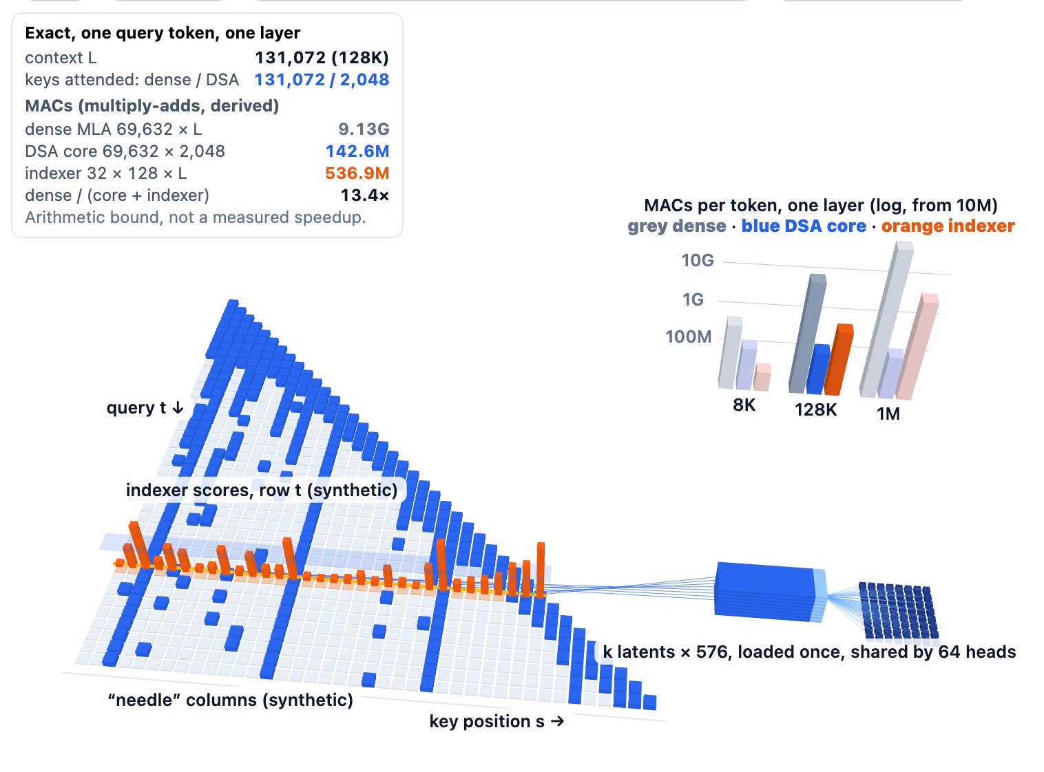
Where the cost goes. Sparse attention costs the same at every context length beyond 2,048: 64 heads × 1,088 × 2,048 ≈ 142.6M multiply-adds per query token per layer. The indexer grows by 4,096 per earlier token, so it overtakes the sparse attention at about 34,800 tokens (both derived):

Context $L$	Dense MLA attention	Indexer scoring	Sparse attention ($k$ = 2,048)	Dense ÷ (indexer + sparse)
8K (8,192)	0.57G	0.03G	0.14G	3.2×
128K (131,072)	9.13G	0.54G	0.14G	13.4×
1M (1,048,576)	73.0G	4.29G	0.14G	16.5×

Multiply-adds per query token per layer, all derived from the config. These are arithmetic upper bounds on attention work, not speedups. Real cost also depends on memory bandwidth, kernel efficiency, batching and the rest of the model. For comparison, the GLM-5 report, citing DeepSeek-V3.2’s experience, says DSA “reduces the attention computation by roughly 1.5-2× for long sequences” and lets the model “handle 128K contexts at half the GPU cost.”

The table also shows the catch: at 1M the indexer is about 97% of DSA’s attention work. Past a few tens of thousands of tokens, the cheap scorer is what DSA’s cost scales with. §5.5 measures that on real hardware, and §5.6 is GLM-5.2’s answer.

Implementation notes and memory traffic

• Top-k. Miles’ default backend is plain torch.topk(logits, 2048); positions whose score is $-\infty$ become index −1. An optional FlashInfer backend has a determinism switch. Miles hard-codes index_topk = 2048 instead of reading it from the config.
• Sparse kernel. Each head’s absorbed query is 576 wide and the key-value cache has a single group of 576-wide rows (a code comment’s example shows query_absorbed [96, 16, 576] and kv [96, 1, 576]: 16 heads on one rank sharing a single 576-wide KV group). The TileLang SparseMLA kernel asserts a 576-wide key and a 512-wide value, requires the top-k count to be a multiple of 64, loads zeros and scores $-\infty$ for index −1, and passes no gradient to the indices. The output is multiplied by $W^{UV}$ afterwards (einsum("thm,hdm->thd", out, w_vc)).
• Ascend. The GLM-5 report also describes a fused “Sparse Flash Attention” kernel that selects the top-k tokens from the KV cache and computes sparse attention in parallel.
• Decode memory traffic (derived; assumes a bf16 cache, which the sources do not specify). Per layer, dense decoding reads $L$ × 1,152 bytes of latent cache. DSA reads 2,048 × 1,152 bytes of selected latents plus $L$ × 256 bytes of index keys. That is 2.1× less at 8K, 4.2× at 128K and 4.5× at 1M. The ratio cannot exceed 1,152 / 256 = 4.5×, because the index keys themselves grow with $L$; an FP8 index key would double that cap. By our reading, this is why the size of the index key, not $k$, bounds DSA’s decode savings.
• Arithmetic. 2,048 / 1,048,576 = 0.195%; break-even 142.6M / 4,096 ≈ 34,800 tokens. Both are ours.

5.4 How DSA is trained: a dense warm-up, then sparse training

DSA is not trained from scratch. Both DeepSeek-V3.2 and GLM-5 started from a dense MLA model and switched it to sparse attention with a short continued pre-training. The problem to solve is that a fresh indexer knows nothing, and if its random picks were used right away, the model would attend to the wrong tokens.

The fix is to teach the indexer by imitation first. The dense model already “knows” which tokens matter: its attention weights say so. DeepSeek-V3.2’s recipe has two stages.

Stage 1, dense warm-up. Attention stays dense, and every parameter except the lightning indexer is frozen. For each query token $t$, the main attention scores are summed across all heads and normalized along the sequence (L1) into a distribution $p_{t,:}$. The indexer is trained to match it with a Kullback–Leibler (KL) divergence loss:

\[\mathcal{L}^{I}=\sum_t D_{\mathrm{KL}}\!\Big(p_{t,:}\;\Big\|\;\mathrm{Softmax}\big(I_{t,:}\big)\Big)\]

In plain terms: if the 64 attention heads together put 30% of their weight on token 812 and 10% on token 40,000, the indexer is pushed to give token 812 the higher score. The softmax appears only in this loss; at inference the scores are just sorted. DeepSeek ran this for 1,000 steps of 16 sequences × 128K tokens (2.1B tokens) at a learning rate of 1e-3.

Stage 2, sparse training. Top-k selection is switched on, and all parameters are trained so that the model adapts to seeing only 2,048 tokens per query. The indexer keeps its KL target, now restricted to the selected set $S_t$ (the 2,048 positions it picked):

\[\mathcal{L}^{I}=\sum_t D_{\mathrm{KL}}\!\Big(p_{t,S_t}\;\Big\|\;\mathrm{Softmax}\big(I_{t,S_t}\big)\Big)\]

The two halves learn from separate signals. In DeepSeek’s words, “we detach the indexer input from the computational graph for separate optimization. The training signal of the indexer is from only $\mathcal{L}^I$, while the optimization of the main model is according to only the language modeling loss.” Stage 2 used 15,000 steps of 480 sequences × 128K tokens (943.7B tokens) at a learning rate of 7.3e-6, and V3.2’s post-training also ran sparse.

Our reading of the division of labor: the top-k choice is not differentiable, so the language-model loss could not teach the indexer anyway. The KL loss teaches it to rank well, while the backbone learns to live with whatever was picked.

The DSA 3D model in §5.3 has a mode for each of the two stages.

How GLM-5 adapted the recipe. GLM-5 followed the same two stages, starting from “the base model at the end of mid-training,” which had used dense MLA throughout:

	DeepSeek-V3.2	GLM-5
Starting point	V3.1-Terminus base, already extended to 128K	end of mid-training (dense MLA)
Warm-up	1,000 steps × 16 × 128K ≈ 2.1B tokens, LR 1e-3	1,000 steps × 14 × 202,752 ≈ 2.84B tokens, LR 5e-3 → 2e-4
Sparse stage	943.7B tokens, LR 7.3e-6	20B tokens, mid-training data and hyperparameters, constant LR 1e-5

GLM-5’s sparse stage is about 2% of DeepSeek’s (by our count). The report says that “although the training budget is much smaller than that of DeepSeek-V3.2 (943.7B tokens), we find that it is enough to adapt the DSA model to match the performance of the original MLA model.”

The evidence. The report’s Table 3 compares the MLA and DSA base models at 128K on two needle-in-a-haystack retrieval tests (multi-query and multi-value) and two question-answering sets:

128K test	MLA	DSA
MQ-NIAH	100.0	100.0
MV-NIAH	95.5	97.0
SQuAD	79.7	86.0
HotpotQA	66.3	63.0

That is a rough tie, with DSA ahead on some tasks and behind on others. After the same supervised fine-tuning (SFT) data, the report says “the two models tie in training loss and evaluation benchmarks.”

The report also calls DSA “lossless by construction.” Treat that phrase as the authors’ framing: top-k selection does drop tokens for each query.

A smaller experiment in the same report shows both why the second stage matters and where a gap remains. GLM-4.7-Flash (30B, MLA) received an indexer-only warm-up of 1,000 steps, then 150B tokens of joint training. On RULER, the warm-up alone lost 7.86 points at 128K; joint training recovered most of it, beating the original model by 0.49 to 1.72 points at 16K to 64K but still trailing by 0.35 at 128K.

What we do not know for GLM-5.3. No source describes how GLM-5.3’s DSA was trained. GLM-5.3 shares GLM-5.2’s base model, and the GLM-5.2 card does not describe its DSA training either. The recipe above is GLM-5’s. The Miles framework, which does RL post-training, does not reproduce either KL loss; it keeps the indexer out of RL updates (§10; GLM-5’s own RL choice is in §5.7).

Where the numbers come from

• DeepSeek-V3.2 recipe: V3.2 paper, Sec. 2.1 (Eq. 3 and 4, learning rates, step counts, token totals). 1,000 × 16 × 131,072 ≈ 2.1B and 15,000 × 480 × 131,072 ≈ 943.7B match the paper’s totals. The paper does not say whether $p_{t,S_t}$ is renormalized over $S_t$ in stage 2.
• GLM-5 recipe: GLM-5 report, Sec. 2.1.1 and Appendix A (learning-rate schedule). The warm-up total (1,000 × 14 × 202,752 ≈ 2.84B) and 20 / 943.7 ≈ 2.1% are our arithmetic. The GLM-5 section does not say explicitly that only the indexer trains during warm-up; the report calls indexer-only warm-up the “standard DSA recipe” in its GLM-4.7-Flash experiment.
• Table 6 (RULER, GLM-4.7-Flash plus DSA): base 79.21 at 128K, warm-up only 71.35, after 150B joint tokens 78.86. Deltas +0.86 at 16K, +0.49 at 32K, +1.72 at 64K, −0.35 at 128K.
• The report’s statement that DeepSeek-V3.2-Exp proved “90% of attention entries in long contexts are indeed redundant,” and the 1.5–2× figure, are GLM-5’s wording; we did not find them in the V3.2 paper.
• Miles: no indexer KL loss in the GLM-5 or Flash paths (the indexer’s scores are computed and discarded after top-k); a --freeze-indexer flag sets requires_grad to False on the indexer projections.

So DSA reads only 2,048 tokens per query, at little cost in quality. The catch is that the indexer itself still scores all $L$ earlier tokens for every query, so it remains $O(L^2)$. In GLM-5 and GLM-5.1, it ran independently in all 78 layers. That cost is what §5.5 and §5.6 are about.

5.5 When the indexer becomes the bottleneck

Sparse attention makes reading cheap: at most 2,048 tokens per query, no matter how long the context grows. Choosing is still expensive, because the indexer must score every earlier token, in every layer. The arithmetic in §5.3 put the crossover near 35K tokens for GLM-5.3’s sizes; measurements on a smaller DSA model point the same way.

The IndexCache paper measured this on a 30B DSA model (built from GLM-4.7-Flash, 47 layers). From the chart labels, the indexer’s share of prefill latency grows from about 27% at 10K tokens to roughly 80% at 200K; for decode it grows from about 27% to about 41%. By that reading, at 200K the cheap scorer takes more prefill time than the rest of the model combined.

The same paper found the waste to cut. Comparing the 2,048 tokens each layer selects, adjacent layers share 70–100% of their picks, and some runs of layers form clusters with mutually high overlap. If layer 7 would select almost the same tokens as layer 6, layer 7 does not need its own indexer.

Where the numbers come from

• Latency shares: IndexCache paper, profiling chart in the introduction. We read the values (prefill 27/50/68/81%, decode 27/31/38/41% at 10K/60K/120K/200K) from the chart text extracted from the PDF, so treat the exact mapping as our reading.
• Overlap: IndexCache Appendix A, overlap = the size of T(i) ∩ T(j) divided by 2,048, averaged over 768 samples of 200K length on the 47-layer model. Early and late layers overlap at most about 0.4.

5.6 IndexShare: one indexer for every four layers

GLM-5.2 introduced the fix, and GLM-5.3 inherits it unchanged. The GLM-5.2 model card calls it IndexShare; the paper it links (arXiv 2603.12201, by Tsinghua and Z.ai authors) calls the same method IndexCache. The idea fits in two lines:

• Full (F) layers, the “compute” layers of §1.2, run their own indexer, pick the top 2,048 tokens, and store that index list in a buffer.
• Shared (S) layers, the “reuse” layers, have no indexer. They reuse the list from the nearest F layer before them.

In inference this costs “a single conditional branch.” The buffer holds only the current index tensor and is overwritten at each F layer, so the paper says it “requires no additional GPU memory beyond what standard DSA already allocates.”

The 3D model below shows where the shared layers sit in the stack.

Scroll a 3D landscape of layers against past keys and watch which keys each attention layer reads: GLM-5 runs its key-choosing indexer on all 78 layers, GLM-5.3 on only 21 (IndexShare), and GLM-5.3-Flash on 11 of 45 over 4-token pools. Use the model and context toggles (8K to 1M) and hover or tap layers for details; layer roles and counts are exact, score shapes are synthetic.

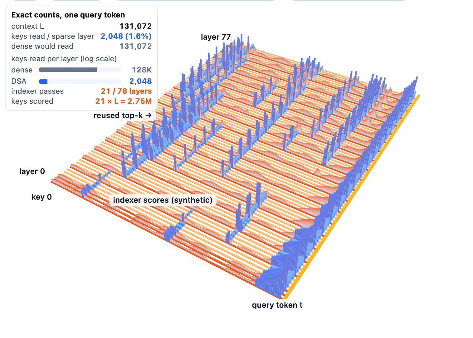
The GLM-5.2 / GLM-5.3 layout. The config’s indexer_types list applies the §2.2 rule: 21 full and 57 shared layers, which in the paper’s F/S notation reads FFFSSS, then FSSS eighteen more times. The GLM-5.2 card states the payoff as “reducing per-token FLOPs by 2.9x at a 1M context length.” That is Z.ai’s claim; the card does not name the baseline, though our reading is that it compares against GLM-5.1’s every-layer indexer.

S layers are not just switched off. GLM-5.3’s FP8 config lists indexer tensors (such as the indexer’s key LayerNorm) only for the 21 F layers plus layer 78, the MTP layer from §2, so by that evidence shared layers carry no indexer parameters at all.

What the paper measured. These numbers come from the IndexCache paper’s own models, not from GLM-5.2 or GLM-5.3:

Model and setting	Result
30B DSA model, keep 1/4 of indexers, 200K context	Prefill 19.5 s → 10.7 s (1.82×); per-request decode 58 → 86 tokens/s (1.48×)
744B GLM-5, training-free, keep 1/4, searched layers	Long-context average 78.0 vs 78.4 for full DSA
744B GLM-5, training-free, keep 1/4, uniform layers	Long-context average 72.7
744B GLM-5, keep 1/4, beyond 100K context	“at least 1.3×” in prefill latency and decode throughput
30B, training-aware, keep 1/4, uniform layers	Long-context average 50.6 vs 51.0 for full DSA

The two GLM-5 rows carry the paper’s main lesson for the training-free case: “which indexer layers are retained matters far more than how many.” Choose the wrong quarter of layers and long-context quality drops by almost 6 points. On the 30B model, the training-aware method closes that gap. It trains each surviving indexer to match the averaged attention of all layers it serves, and with it even a simple uniform pattern lands within half a point of full DSA.

That raises a question the sources leave open. GLM-5.2 and GLM-5.3 ship a uniform pattern, not either of the paper’s irregular searched GLM-5 patterns, even though uniform did badly training-free. Our reading is that the 5.2 base was likely trained with sharing in place, in the training-aware style. Neither model card says so, and the paper listed training-aware IndexCache for GLM-5 only as future work.

The parameter effect is tiny. Dropping 57 indexers saves about 0.534B parameters (by our count), roughly 0.07% of the model. IndexShare is a compute and latency optimization, not a size one; Flash attacks the same choosing cost by pooling (§8.5).

Implementation notes

• Config keys. index_topk_freq 4 and index_skip_topk_offset 3 first appear in GLM-5.2 and are identical in GLM-5.3, as is the 78-entry indexer_types list. GLM-5 and GLM-5.1 have none of these keys, so every layer there runs its own indexer.
• Pipeline constraint. Miles keeps the shared top-k in a per-microbatch holder that does not cross pipeline stages, so every pipeline stage must start on a computing layer. In its GLM-5.2 script, the largest layout uses 8 pipeline stages with 14 layers in the first stage and 16 in the last, so stages start at layers 1, 15, 23, 31, 39, 47, 55, 63 (1-indexed), all computing layers. The 64-GPU GB300 layout uses 4 stages split 18 / 20 / 20 / 20, so stages start at 1, 19, 39, 59.
• FP8 evidence. The indexer entries in modules_to_not_convert exist for 22 layers: the 21 full layers plus layer 78 (MTP). The list also names a tensor self_attn.indexers_proj, which does not match Miles’ tensor names; we have not checked it against the safetensors index.
• Counting. 21 / 78 = 26.9% and 57 / 78 = 73.1% count main-stack layers only. Including the MTP layer’s own indexer, 22 of 79 positions run one (27.8%).
• Undocumented keys. index_topk_pattern is null and index_share_for_mtp_iteration is true; neither is documented in our sources (see §6).

5.7 A footnote for RL: the top-k must be deterministic

6. Long Context, MTP, and FP8 Packaging

Three more things separate GLM-5.3 from the original GLM-5: a five-times longer context window, a better draft layer for speculative decoding, and weights shipped in 8-bit floating point. The first two arrived with GLM-5.2. The third is a packaging choice that leaves the architecture untouched.

	GLM-5 / GLM-5.1	GLM-5.2 / GLM-5.3
max_position_embeddings	202,752	1,048,576
rope_theta	1,000,000	8,000,000
rope_scaling / YaRN	none	none (rope_type “default”)
MTP layers (num_nextn_predict_layers)	1	1
index_share_for_mtp_iteration	absent	true
quantization_config	absent	GLM-5.3 only: FP8 e4m3

6.1 One million tokens

The first two rows of the table moved together in GLM-5.2: the window grew to 1,048,576 ($2^{20}$, “1M”) positions, a 5.17× jump (derived), and the rotary base rose eightfold with no rope_scaling entry. Our reading is that this is plain base-frequency scaling: a larger base slows the rotation of the 64 RoPE dimensions (§3.3), so positions far apart stay distinguishable. The GLM-5.2 card describes the result as delivering long-horizon capability “on a solid 1M-token context.”

How the model was trained to use that window is not documented. The closest public recipe is GLM-5’s mid-training, which extended context in three stages: 32K (1T tokens), then 128K (500B tokens), then 200K (50B tokens). Nothing in our sources describes a corresponding stage for 1M.

6.2 Multi-token prediction

MTP adds a small extra layer that guesses the next few tokens. At inference those guesses serve as drafts for speculative decoding: the main model verifies several drafted tokens in one pass and keeps the ones it agrees with. GLM-5.3 has one such layer, layer 78 in the checkpoint, with the structure described in §2.

GLM-5 shares the parameters of three MTP steps during training. The report says this keeps the draft model’s memory cost at DeepSeek-V3’s level while lifting the average accepted length above DeepSeek-V3.2’s (details below).

GLM-5's MTP training trick

The GLM-5 report explains its MTP training trick. DeepSeek-V3 trains one MTP layer but uses it to predict two tokens at inference, and that mismatch lowers acceptance of the second token. GLM-5 instead shares the parameters of three MTP steps during training. This keeps the draft model’s memory cost the same as DeepSeek-V3’s, but acceptance rises: with 4 speculative steps on a private prompt set, the average accepted length is 2.76 for GLM-5 vs 2.55 for DeepSeek-V3.2.

GLM-5.2’s card adds that it improved the MTP layer, “increasing the acceptance length by up to 20%.” The config shows no structural change: there is still exactly one MTP layer. The only new MTP-related key is index_share_for_mtp_iteration, set to true. Our reading is that the 5.2 gain came mostly from training, and that the flag may let the MTP layer reuse one indexer selection across drafting steps. Neither the card nor Miles documents the flag, so treat both points as interpretation.

6.3 FP8 packaging

GLM-5.3’s one substantive config change, the quantization_config block, describes an FP8 checkpoint:

• Format: FP8 e4m3 (4 exponent bits, 3 mantissa bits).
• Weights: quantized in blocks of 128 × 128, each block with its own scale.
• Activations: quantized dynamically at run time (activation_scheme “dynamic”).
• Kept in higher precision: 541 entries in modules_to_not_convert.

The exceptions are the small or sensitive pieces: the norms, the MoE router gate and its expert bias, the embeddings, the lm_head, and a few MTP and indexer tensors (the notes below list them). Everything with real bulk is FP8, including the attention projections, the indexer’s query and key projections (wq_b, wk), the dense MLPs, and all experts. This changes storage and serving cost, not the network: same layers, same shapes, same IndexShare layout.

Implementation notes

• Counting the 541. Three non-layer entries (lm_head, model.norm, model.embed_tokens). Four norms per layer for layers 0–78, MTP included (input_layernorm, post_attention_layernorm, q_a_layernorm, kv_a_layernorm). Router mlp.gate and e_score_correction_bias on the 76 MoE layers 3–78. Three indexer entries on the 22 indexer-bearing layers (§5.6). Four MTP-only entries (eh_proj, enorm, hnorm, shared_head.norm).
• Which repo. The GLM-5.3 config we read carries this FP8 block, while the GLM-5.2 card’s new_version field points to a repository named zai-org/GLM-5.3-BF16. Exactly which Hugging Face variant each file came from is not recorded, and our copy of a separate GLM-5.3-FP8 config was a failed download.
• head_dim 64 → 192. This key changed in GLM-5.2. In GLM-5 it equals the RoPE part of the head (64); in 5.2 and 5.3 it equals the NoPE part (192). The MLA dimensions themselves (qk_nope_head_dim 192, qk_rope_head_dim 64, v_head_dim 256) did not change, so parameter counts are unaffected. We treat it as metadata and do not read more into it.
• Router precision. GLM-5.2 also added moe_router_dtype float32 (§4), which fits with keeping the router gate out of FP8.

7. If the architecture did not change, where did GLM-5.3’s gains come from?

§2–6 described a network that GLM-5.3 inherited unchanged from GLM-5.2. So what improved? Z.ai’s answer is short: the weights did, through more and better post-training. This section reads the model card’s benchmark table carefully, lists the caveats that table carries, and sketches the closest public description of how a GLM-5-family model is post-trained.

The model card says every gain over GLM-5.2 comes from post-training. It claims a “50% improvement over GLM-5.2 on our in-house Z.ai Code Bench,” which outsiders cannot reproduce, and open-source state of the art on Terminal Bench 3.0 and Agents’ Last Exam. It also reports an “Emergent Cyber Capability”: “As we scaled post-training, cyber capability developed faster than we expected.”

7.1 What the benchmark table shows

The table below copies the GLM-5.3 and GLM-5.2 columns from the GLM-5.3 model card. The “Change” column is our own subtraction. The last column names the best of the other six models the card compares against (Kimi K3, DeepSeek-V4 Pro-0813, Qwen3.8-Max, Opus 4.8, Fable 5 with fallback, and GPT-5.6 Sol). Rows where GLM-5.3 is the best of all eight models are marked in bold.

Benchmark (as named in the card)	GLM-5.2	GLM-5.3	Change (derived)	Best other model in the row
Terminal Bench 2.1	81.0	88.2	+7.2	GPT-5.6 Sol, 88.8
Terminal Bench 3.0	4.6	28.3	+23.7	GPT-5.6 Sol, 34.6
DeepSWE (v1.1)	46.2	66.9	+20.7	GPT-5.6 Sol, 72.7
NL2Repo	48.9	58.0	+9.1	Opus 4.8, 69.7
ProgramBench (Almost Solved)	9.5	19.0	+9.5	Fable 5, 33.0
FrontierSWE	67.5	78.1	+10.6	Fable 5, 88.2
SWE-Marathon (v1.1)	19.4	42.5	+23.1	Opus 4.8, 48.8
PostTrainBench	31.7	39.8	+8.1	Fable 5, 41.8
CyberGym	77.2	84.5	+7.3	Fable 5, 83.8
ExploitGym (2h / 6h)	29 / 39	105 / 130	+76 / +91	GPT-5.6 Sol, 216 / 293
ExploitBench	24.4	54.4	+30.0	Fable 5, 78.0
Toolathlon Verified	59.9	73.0	+13.1	Kimi K3, 76.5
AutomationBench (v1.0.6)	26.2	48.2	+22.0	Kimi K3, 46.7
Agents’ Last Exam (ALE-CLI)	23.8	28.5	+4.7	GPT-5.6 Sol, 28.6
HLE w/ Tools	54.7	62.5	+7.8	GPT-5.6 Sol, 64.5
GDPval-AA v2	1,508	1,769	+261	Fable 5, 1,743

GLM-5.3 improves on GLM-5.2 in all 16 rows. The largest relative jumps (ratios are our arithmetic) sit in long-horizon agent work and security: about 6× on Terminal Bench 3.0, about 3.6× on ExploitGym at the 2-hour budget, about 2.2× on SWE-Marathon and ExploitBench, 2× on ProgramBench, and about 1.8× on AutomationBench.

These match the card’s two headline claims: better long-horizon coding, and cyber skill that “more than doubles GLM-5.2 on exploitation benchmarks.”

Read against the whole field, the picture is more modest. GLM-5.3 is the best of the eight models in only three rows: CyberGym, AutomationBench, and GDPval-AA v2. The card’s “open-source SOTA” claim rests on two benchmarks, and on both a closed model scores higher: Fable 5 (33.7) and GPT-5.6 Sol (34.6) beat GLM-5.3’s 28.3 on Terminal Bench 3.0, and GPT-5.6 Sol edges it on Agents’ Last Exam (28.6 vs 28.5). So the qualifier “open-source” is doing real work; the table supports the claim as worded, not as “best overall.”

Where the numbers come from

• All scores are copied from the benchmark table in the GLM-5.3 model card; bold there marks the best score in each row. The change column, the ratios, and the “best other model” column are our arithmetic on that table.
• The card does not use one unit across rows. GDPval-AA v2 is not a percentage (scores sit around 1,500–1,800), and ExploitGym reports two numbers, one per time budget (2 hours and 6 hours) on its 869 tasks. We subtract within each row only.
• Harness settings differ by row and come from the card’s footnotes. Several rows (Terminal Bench 2.1, Terminal Bench 3.0, CyberGym, ExploitGym, ExploitBench, PostTrainBench, SWE-Marathon) run GLM-5.3 inside Claude Code 2.1.207. Terminal Bench 3.0 uses a 400K context, 128K maximum output, avg@3 (the mean of three runs per task), a 600-turn cap, and a 10-hour timeout. CyberGym is a single-run Pass@1 (one attempt per task, scored once) over 1,507 tasks with unlimited time per task and a domain whitelist. FrontierSWE was run by Proximal, and its dominance score (a relative score against the other models evaluated) is dated 2026/08/14.

7.2 Caveats before you quote these numbers

Three smaller cautions:

• The headline coding number is in-house. The 50% gain on Z.ai Code Bench has no public task set.
• Single runs. CyberGym and ExploitGym are reported as single-run Pass@1, so run-to-run variance is unknown.
• The row set changed. The GLM-5.3 card drops several GLM-5.2 rows, including the pure reasoning and math rows, and the card does not say how 5.3 does on them (details below).

Main cross-card mismatches

GLM-5.2 scores that match in both cards: Terminal Bench 2.1 (81.0), DeepSWE (46.2), NL2Repo (48.9), and HLE w/ Tools (54.7). Scores that differ (GLM-5.2 card → GLM-5.3 card):

Benchmark	GLM-5.2 card	GLM-5.3 card	Likely cause (our reading)
FrontierSWE	74.4	67.5	Dominance is a relative score dated 2026/06/16 vs 2026/08/14; it moves as new models join
PostTrainBench	34.3	31.7	Different protocol: the 5.3 card self-runs and falls back to the zero-shot baseline on failed runs
SWE-Marathon	13.0	19.4	The 5.3 card uses v1.1
ProgramBench	63.7	9.5	Different metric (“Almost Solved” in the 5.3 card)
Tool-Decathlon → Toolathlon Verified	48.2	59.9	The 5.3 card reports a renamed or re-verified version of the benchmark

Two more notes, both our reading. The Terminal Bench 2.1 “match” is numeric only: 81.0 is the Terminus-2 row in the GLM-5.2 card, while the 5.3 card says it ran Terminal Bench 2.1 in Claude Code. The 5.3 card also drops MCP-Atlas, CritPt, and IMOAnswerBench, which the 5.2 card reported.

Compared with the GLM-5.2 card, the GLM-5.3 card drops the pure reasoning and math rows and SWE-bench Pro, and adds Terminal Bench 3.0, three cyber benchmarks, AutomationBench, Agents’ Last Exam, and GDPval-AA v2. Our reading is that post-training effort moved toward agentic, long-horizon, and security work.

7.3 What “post-training” means for this family

Z.ai has published no GLM-5.3 technical report, so nobody outside knows its exact recipe. The closest documented method is the GLM-5 technical report, which the GLM-5.3 and GLM-5.3-Flash cards both cite. Treat what follows as the family’s public recipe, not a confirmed account of GLM-5.3’s training. For GLM-5, post-training runs in five stages: SFT, reasoning RL, agentic RL on more than 10,000 verifiable software-engineering and terminal environments, general RL, and on-policy cross-stage distillation, which keeps later stages from erasing earlier skills.

The five GLM-5 post-training stages in detail

1. Supervised fine-tuning (SFT). Multi-task data covering general chat, reasoning, and coding and agent work, with up to 202,752 tokens of context. The model learns three thinking modes: interleaved (think before every reply and tool call), preserved (keep earlier thinking blocks across turns in coding agents), and turn-level (switch thinking on or off per turn). Erroneous steps in agent trajectories stay in the data but are masked out of the loss.
2. Reasoning RL. RL with GRPO (Group Relative Policy Optimization) plus IcePop over math, science, code, and tool-integrated reasoning. IcePop drops tokens whose training-to-inference probability ratio falls outside $[1/\beta, \beta]$, with $\beta = 2$, and the clip range is $\epsilon_{\text{low}} = 0.2$, $\epsilon_{\text{high}} = 0.28$.
3. Agentic RL. Fully asynchronous RL on more than 10,000 verifiable software-engineering and terminal environments plus multi-hop search tasks. A token-in-token-out (TITO) gateway avoids re-tokenization mismatches, and double-sided importance sampling masks tokens whose ratio to the rollout policy leaves $[1-\epsilon_l, 1+\epsilon_h]$.
4. General RL. Rule-based rewards, outcome reward models, and generative reward models, with human-written responses as style anchors.
5. On-policy cross-stage distillation. The final checkpoints of earlier stages act as teachers, so later stages do not erase earlier skills.

In plain terms: with $\beta = 2$, a token survives the IcePop filter only if the training engine assigns it between half and twice the probability the inference engine gave it when sampling. Anything outside that band is treated as a training-inference mismatch and contributes no gradient.

The two RL safeguards of §5.7, a frozen indexer and a deterministic top-k, come from this same recipe and tie it back to the architecture. Our reading: sparse attention adds a second “routing” decision, besides MoE routing, that RL must keep stable.

The GLM-5.3 card’s emphasis (terminal work, multi-hour software tasks, exploitation chains) lines up with the agentic RL stage and its environment scaling. That alignment is our interpretation; the card says only that the gains come from scaled post-training. For how the mechanics work in an open framework (TITO, routing replay, importance-sampling corrections, fully async training), see our earlier Miles deep dive.

8. GLM-5.3-Flash: A New Hybrid, Not a Smaller GLM-5.3

GLM-5.3-Flash shares a name, a vocabulary, and a release day with GLM-5.3, but it is a different machine. This section answers one question: what did Z.ai change when it designed a model from scratch for cheap long-context serving? The short answer is that most layers trade the ever-growing attention cache for a small memory of fixed size, while every fourth layer keeps exact, sparse attention for precise lookups.

The model card is explicit about the break. Flash “starts from a newly trained base model”, and “for the first time in the GLM series” it uses “a hybrid architecture combining sparse and linear attention”. It also “adopts Manifold-Constrained Hyper-Connections (mHC)” and was pre-trained on Z.ai’s “latest 30T-token multimodal pre-training corpus”. The card gives 320B total and 18B active parameters.

The Miles documentation says the same thing in engineering terms: Flash “is a different architecture from the 744 B GLM5 and GLM5.2 flagships, not a smaller cut of them.”

8.1 The Layout: Three KDA Layers, Then One DSA Layer

Flash has 45 transformer layers, against GLM-5.3’s 78, and a narrower hidden size (4,096 against 6,144). Two kinds of attention alternate in a fixed rhythm:

• KDA, a linear-attention layer with a fixed-size memory, at 34 layers.
• DSA, the sparse attention from GLM-5.3 (§5), at 11 layers. An indexer still picks 2,048 tokens per query, but here it scores pooled blocks of four tokens (§8.5).

The pattern is [KDA, KDA, KDA, DSA] repeated 11 times, which gives 44 layers, plus one trailing KDA layer (layer 44). DSA sits at layers 3, 7, 11, …, 43, that is, every layer whose index leaves remainder 3 when divided by 4. Within each block of four the ratio is 3:1; over the whole stack it is 34:11.

The feed-forward side follows GLM-5.3’s convention, dense in layers 0–2 and MoE after, so layer 3 is both the first DSA layer and the first MoE layer.

Layers	Attention	FFN
0, 1, 2	KDA	dense (12,288)
3, 7, 11, …, 43 (11 layers)	DSA: NoPE MLA + pooled indexer	MoE
4–6, 8–10, …, 40–42, and 44 (31 layers)	KDA	MoE
45 (MTP, extra)	DSA with its own indexer	MoE

Two more pieces wrap this stack. mHC widens the residual path into four streams mixed at both sublayers of every layer, 90 mixing sites in all (§8.6). The MTP layer 45 in the table has no mHC parameters in the checkpoint’s name list, so our reading is that it is not wrapped in mHC; Miles drops it for training.

To walk through this stack layer by layer, switch the layer-stack 3D model in §2.2 to Flash mode.

Where the numbers come from

• text_config.layer_types in the Flash config.json lists 34 "linear_attention" and 11 "deepseek_sparse_attention" entries; linear_attn_config.kda_layers and linear_attn_config.full_attn_layers repeat the same split (DSA = [3, 7, …, 43]).
• Miles (miles_plugins/models/glm5_next/glm5_next.py, full_attn_layers()) reads full_attn_layers, falls back to layer_types, and defaults to i % 4 == 3. Layers in that set get Glm5NextDSAAttention; all others get Glm5NextKDAAttention.
• FFN types: first_k_dense_replace = 3, mlp_layer_types = 3 × "dense" + 42 × "sparse", intermediate_size = 12288.
• MTP: num_nextn_predict_layers = 1. The FP8 skip list (quantization_config.modules_to_not_convert) shows model.layers.45.* with self_attn.indexer.*, kv_b_proj, mlp.gate, and eh_proj/enorm/hnorm, but no hc_attn_*/hc_ffn_* entries. Layers 0–44 all have them.
• Miles docs (docs/models/glm/glm5-3-flash.md): “MTP is dropped for training.”

8.2 KDA: Linear Attention with a Fixed-Size Memory

Ordinary softmax attention keeps every past key and value, so its cache grows by one entry per token, forever. KDA instead keeps a small matrix per head, a notebook of fixed size, and rewrites it in place as each token arrives. Reading the notebook costs the same at token 10 as at token 1,000,000. The animation below contrasts the two.

A KDA layer keeps one 128 × 128 state per head, decays it per channel and rewrites it in place with the delta rule (the published KDA form), while a softmax layer's cache grows with every token. Memory numbers are our bf16 estimates for one sequence of one million (10⁶) tokens, as in §9, and ignore FP8 KV and indexer caches. Open the full-size SVG.

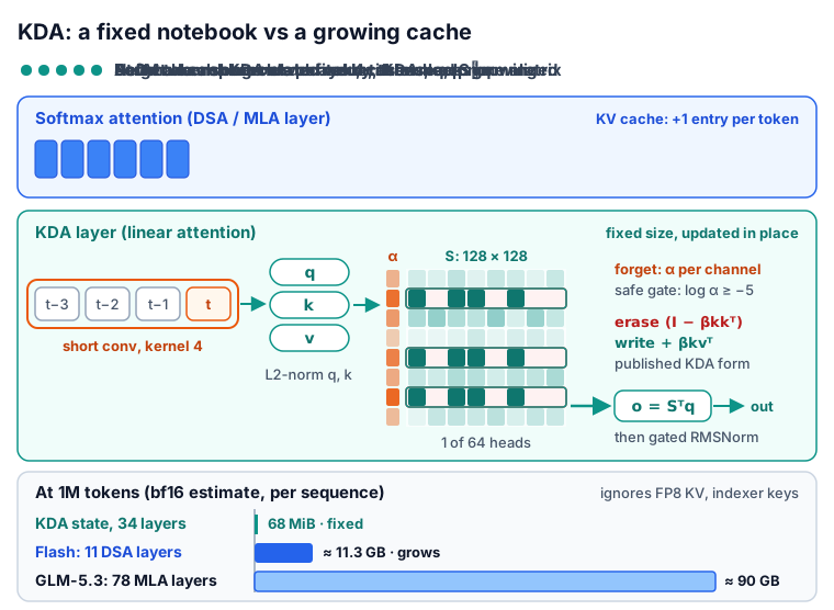
KDA comes from Moonshot AI’s Kimi Linear paper (arXiv 2510.26692). It is the last step of a short lineage: linear attention, then the delta rule, then a forget gate, then a finer forget gate. The subsections below take these steps one at a time, then cover the full layer in Flash, how it trains, how it decodes, and why Flash mixes it with DSA.

8.2.1 Linear Attention: A State Instead of a Cache

Softmax attention scores the current query $q_t$ against every past key $k_i$, normalizes the scores, and averages the values $v_i$. The softmax couples all past tokens, so they must all stay in memory.

Drop the softmax and the sum factorizes. The output becomes $o_t = \sum_{i \le t} (q_t^\top k_i)\, v_i = S_t^\top q_t$, where $S_t = \sum_{i \le t} k_i v_i^\top$. The past is now summarized by one matrix $S_t$ of size $d_k \times d_v$, updated by adding one outer product per token:

\[S_t = S_{t-1} + k_t v_t^\top, \qquad o_t = S_t^\top q_t\]

In plain terms, $S$ is a key-value memory. Writing stores $v_t$ “under” the direction $k_t$; reading with a query returns the values stored under similar directions. With $d_k = d_v = 128$, as in Flash, the memory holds 16,384 numbers per head, whatever the sequence length.

The flaw is that this memory only adds. It never erases, and a 128-dimensional key space has room for at most 128 mutually orthogonal keys. After thousands of writes, every read returns a blurred sum of many values. The Kimi Linear paper describes plain linear attention as having “no criterion for which memories to erase”, with a state that “grows unbounded”.

8.2.2 The Delta Rule: Write Only the Error

The delta rule fixes the “only adds” flaw. Before writing, the layer asks what the memory currently returns for the key, $\hat v_t = S_{t-1}^\top k_t$. It then writes only the difference between the target and that prediction, scaled by a write strength $\beta_t \in (0, 1)$:

\[S_t = S_{t-1} + \beta_t\, k_t \left(v_t - S_{t-1}^\top k_t\right)^\top = \left(I - \beta_t k_t k_t^\top\right) S_{t-1} + \beta_t k_t v_t^\top\]

This is one step of gradient descent on the reconstruction error $\tfrac12 \lVert S^\top k_t - v_t \rVert^2$, with $\beta_t$ as the learning rate. It is the update of DeltaNet, and the Kimi Linear paper presents plain linear attention in the same gradient-descent view.

A tiny example makes the difference concrete. Take $d_k = 2$ and one-number values, so $S$ is a column of two numbers, starting at zero.

Step	Write (key → value)	Linear attention $S$	Delta rule $S$ ($\beta = 1$)
1	$(1, 0) \to 3$	$(3, 0)$	prediction 0, error 3: $(3, 0)$
2	$(1, 0) \to 5$ (the fact changed)	$(8, 0)$	prediction 3, error 2: $(5, 0)$
3	$(0.6, 0.8) \to 1$	$(8.6, 0.8)$	prediction 3, error −2: $(3.8, -1.6)$

After step 2, querying with $(1, 0)$ returns 8 from linear attention, a sum of the stale and the new fact, but exactly 5 from the delta rule. With $\beta = 0.5$ the delta rule would move only halfway, to 4.

After step 3, the delta rule returns exactly 1 for the new key ($0.6 \times 3.8 - 0.8 \times 1.6 = 1$). The old fact drifts from 5 to 3.8 because the two keys overlap. A finite memory still interferes; with $\beta = 1$ the delta rule makes the newest write exact; with a smaller $\beta$ it moves part of the way, but errors still do not pile up the way plain sums do.

Why the update is stable

• KDA L2-normalizes every key, so $\lVert k_t \rVert = 1$. Then $I - \beta_t k_t k_t^\top$ has eigenvalue $1 - \beta_t$ along $k_t$ and 1 in every other direction: it shrinks the memory only along the key being written and never amplifies anything. The paper cites L2 normalization “to ensure eigenvalues stability”.
• The Kimi Linear paper calls this rank-1 update “equivalent to a generalized Householder transformation”, and notes that it “supports hardware-efficient chunkwise parallelization” (§8.2.5).
• Plain linear attention is gradient descent on the unbounded objective $-\langle S^\top k_t, v_t \rangle$, which explains why it never erases.

8.2.3 Gates: From One Fade per Head to One Fade per Channel

The delta rule corrects facts it is asked about, but it never forgets anything else. Gated DeltaNet (GDN), the linear-attention layer from the §5.1 ablation, adds a forget gate: before each write, the whole state is multiplied by a scalar $\alpha_t \in [0, 1]$ computed from the current token. That is one fade rate per head. The paper reads it as weight decay on the memory.

KDA replaces the scalar with a vector $\alpha_t \in [0, 1]^{d_k}$, one fade rate per key channel. This is the KDA update as published (Eq. 1 of the paper), per head:

\[S_t = \left(I - \beta_t k_t k_t^\top\right) \operatorname{Diag}(\alpha_t)\, S_{t-1} + \beta_t k_t v_t^\top, \qquad o_t = S_t^\top q_t\]

Read it right to left. $\operatorname{Diag}(\alpha_t)$ fades each of the 128 rows of $S$ (one row per key channel, shared by all 128 value columns) by its own factor. The term $(I - \beta_t k_t k_t^\top)$ then erases what the faded memory returns for $k_t$, and $\beta_t k_t v_t^\top$ writes the new value under that key. With $\beta_t = 1$ and a unit-length $k_t$ (KDA normalizes keys), querying with $k_t$ afterwards returns exactly $v_t$, whatever the fade did: the erase step removes everything stored along $k_t$.

Why per channel? The paper’s answer is precision: GDN, “similar to Mamba2, employs a coarse head-wise forget gate”, while the channel-wise gate allows “more precise regulation of the finite-state RNN memory”. A head can keep some channels for long-range facts and let others turn over every few tokens. The paper also reads this gate as a learned, data-dependent positional encoding, which is why Kimi Linear’s own full-attention layers drop RoPE; Z.ai does not say why Flash does the same (§8.3).

The gate in GLM-5.3-Flash, as fla computes it. fla (flash-linear-attention) is the open kernel library whose KDA kernels Miles calls. The layer produces a raw gate value $f_t$ for every head $h$ and channel $c$ through a low-rank projection (4,096 → 128 → 8,192). fla’s fused_kda_gate, called by Miles with lower_bound = -5, turns it into a log-space decay $g$, and the state is multiplied by $\alpha = e^{g}$:

\[g_{t,h,c} = -5 \cdot \sigma\!\left(e^{A_h}\,\big(f_{t,h,c} + b_{h,c}\big)\right), \qquad \alpha_{t,h,c} = e^{\,g_{t,h,c}}\]

Here $\sigma$ is the sigmoid, $A_h$ is the learned A_log (one per head), and $b_{h,c}$ is the learned dt_bias (one per head and channel). Because the sigmoid lies strictly between 0 and 1, $g$ lies in $(-5, 0)$ and $\alpha$ in $(e^{-5}, 1) \approx (0.0067, 1)$.

That is what the −5 lower bound means. Per token, a channel keeps somewhere between 0.67% and 100% of its content: it can fade fast, but no single token can wipe it to exactly zero. fla’s default gate, $-e^{A_h}\,\mathrm{softplus}(f + b)$, has no such floor.

In plain terms, long memory needs $\alpha$ very close to 1, which means a sigmoid output near 0 (derived from the formula; trained values are not in our sources):

Per-token keep factor $\alpha$	Half-life (tokens)	Sigmoid output needed
0.0067 (the floor)	under 1	→ 1
0.082	under 1	0.5 (raw input 0)
0.99	about 69	0.002
0.999	about 693	0.0002
0.9999	about 6,931	0.00002

The half-life is $\ln 0.5 / \ln \alpha$. The second row is the neutral point: with $A_h = 0$ (Miles’ initial value) and $f + b = 0$, $g = -2.5$ and $\alpha \approx 0.082$.

Implementation notes

• Gate code: ops/kda/gate.py in fla at commit 8024667ab58f. The Triton kernel computes lower_bound * sigmoid(exp(A_log) * (g + dt_bias)) when a lower bound is given and -exp(A_log) * softplus(g + dt_bias) otherwise. Miles requires fla ≥ 0.4.2 and pins no commit, so the exact version GLM trained with is not certain.
• fla’s chunk_kda docstring: the bound “naturally clamps the output to [lower_bound, 0)”; “Recommended value: -5 (i.e., per-step decay exp(-5) ≈ 0.0067)”. Its safe_gate=True flag also enables “M=16 TensorCore acceleration”. Miles computes the gate outside the kernel and does not pass safe_gate.
• Order of operations in fla’s reference recurrence (ops/kda/naive.py): fade $S$ by $e^{g}$ row by row, then predict with the faded state, then write $\beta_t k_t (v_t - S^\top k_t)^\top$, then read with $q_t$ scaled by $1/\sqrt{128}$ (fla’s default). Expanding the write gives exactly the paper’s Eq. 1.
• The paper specifies only “a decay function $f(\cdot)$ similar to those used in GDN and Mamba”; it gives no lower bound. The −5 comes from the Flash config (gate_lower_bound) and fla.
• Z.ai does not explain why it chose −5. In Miles the bound only shapes the model: it puts a floor under per-token forgetting, and the kernel is not told about it, because safe_gate is not passed. fla’s docstring links the bound to “M=16 TensorCore acceleration”. Our reading: with $g \ge -5$, the cumulative log-decay over 16 tokens is at least −80, so $e^{\pm 80}$ (about $10^{\pm 35}$) stays inside fp32’s range (max about $e^{88.7}$). That would let a kernel factor 16-token blocks into plain matrix multiplications. The code states the clamp and the speedup, not this reasoning.

8.2.4 The Full KDA Layer in GLM-5.3-Flash

Each of Flash’s 34 KDA layers has 64 heads with $d_k = d_v = 128$. Around the update rule sits a ring of small projections, and Miles’ kda.py follows the Kimi Linear design point for point. For a sequence of $T$ tokens:

1. Project. Three linear maps turn the hidden states $[T, 4096]$ into a query, key, and value, each $[T, 8192]$ (64 heads × 128).
2. Short convolution. A causal convolution with kernel size 4, followed by SiLU (the paper’s Swish), mixes each channel of q, k, and v with the same channel of the three previous tokens. This gives every token a little local context before it touches the memory.
3. Split into heads. q, k, and v become $[T, 64, 128]$ each.
4. Write strength. A sigmoid over a 4,096 → 64 projection gives one $\beta_t$ per head: $[T, 64]$.
5. Forget gate. The low-rank 4,096 → 128 → 8,192 projection and the formula of §8.2.3 give one log-decay per head and channel: $[T, 64, 128]$.
6. Update and read. The kernel L2-normalizes q and k, runs the gated delta rule on a $[64, 128, 128]$ state, and returns $[T, 64, 128]$.
7. Output. Each head’s 128 outputs pass through an RMSNorm multiplied by a sigmoid output gate (low-rank again, 4,096 → 128 → 8,192). A final projection maps 8,192 back to 4,096.

The output gate is the paper’s choice too: Kimi Linear uses a low-rank sigmoid gate “to ensure a fair parameter comparison” and to help with “alleviating the Attention Sink”. In its ablation, removing the gate, swapping it for a Swish gate, or removing the short convolution each made perplexity worse (notes below).

Note what is absent: no positional encoding of any kind. Any sense of order must come from the convolution window, the decay, and the order of the recurrent writes themselves (§8.3).

Tensor	Shape	Notes
q_proj, k_proj, v_proj	4,096 → 8,192 each	no bias
short convolution	24,576 channels × kernel 4	depthwise, SiLU
b_proj ($\beta$)	4,096 → 64	sigmoid
f_a_proj → f_b_proj (forget gate)	4,096 → 128 → 8,192	plus A_log [64], dt_bias [8,192] in fp32
g_a_proj → g_b_proj (output gate)	4,096 → 128 → 8,192	sigmoid, inside the gated RMSNorm
o_proj	8,192 → 4,096
recurrent state (per sequence)	64 × 128 × 128	1,048,576 values

By our count each KDA layer has about 137.7M parameters, nearly all of them (134M) in the four big projections. The 34 KDA layers hold about 3.6 times as many attention parameters as the 11 DSA layers’ MLA blocks (derived).

Implementation notes

• Source: miles_plugins/models/glm5_next/kda.py. Kernels come from fla ≥ 0.4.2: ShortConvolution, FusedRMSNormGated, fla.ops.kda.chunk_kda, and fla.ops.kda.gate.fused_kda_gate.
• Config: linear_attn_config = {num_heads: 64, head_dim: 128, short_conv_kernel_size: 4, gate_lower_bound: -5.0}. Miles refuses to run without the bound: “GLM-5.3 KDA requires gate_lower_bound (safe gate)”.

• Miles runs one convolution over the concatenated 24,576 q

  k

  v channels; the HF checkpoint and fla’s reference layer keep q_conv1d/k_conv1d/v_conv1d separate. Our reading is that the two are equivalent because the convolution acts on each channel independently (fla’s ShortConvolution is a depthwise causal conv; its module is not in our local snapshot).

• The kernel is called with use_qk_l2norm_in_kernel=True. In training it starts from no initial state and discards the final state. The gated norm is FusedRMSNormGated(128, eps=1e-5, activation="sigmoid").
• Small differences from fla’s reference layer: Miles’ output-gate up-projection has no bias (fla’s has one), and Miles initializes A_log and dt_bias to zero. Initial values do not matter for a released checkpoint.
• Kimi Linear ablation (Table 1, training/validation perplexity, lower is better): full design 9.23/5.65; without output gate 9.25/5.67; Swish output gate 9.43/5.81; without convolution 9.29/5.70.
• KDA supports context parallelism in Miles (hybrid_cp = True).
• Parameter count (derived, norm weights excluded): q/k/v 100.7M, o_proj 33.6M, forget and output gates 1.6M each, b_proj 0.26M, convolution 0.1M.

8.2.5 Training in Chunks

Written as a recurrence, KDA processes one token after another. That is fine at inference but wasteful in training, where all $T$ tokens are known in advance and GPUs want large matrix multiplications. The fix is the chunkwise-parallel form; Miles trains KDA this way through fla’s chunk_kda:

1. Cut the sequence into chunks of $C = 64$ tokens (the default in the fla version we read; Miles does not override it).
2. Inside a chunk, compute every token’s interaction with every earlier token of the same chunk at once, as $64 \times 64$ lower-triangular matrices built from dot products of keys and queries, weighted by the cumulative per-channel decay between the two tokens.
3. Pass only the $128 \times 128$ state from one chunk to the next.

The paper calls this “inter-block recurrent and intra-block parallel”. The hard part is step 2: 64 delta-rule updates multiply 64 matrices of the form $(I - \beta k k^\top)\operatorname{Diag}(\alpha)$, which is slow to form naively.

The WY representation solves this. It writes the product of many rank-1 updates as “identity minus a sum of outer products”, so the whole chunk collapses into two small auxiliary matrices $W$ and $U$ computed by matrix multiplications plus one $64 \times 64$ triangular solve. The state then updates once per chunk, and outputs come from two terms: queries reading the incoming state, and a triangular attention-like product inside the chunk. The derivation is below.

Complexity. Per head, chunked KDA costs on the order of $C\,d + d^2$ multiply-adds per token, independent of the sequence length $L$. Dense causal softmax attention costs on the order of $L\,d$ per token. With $C = 64$ and $d = 128$ (derived multiply-add counts, ignoring kernel efficiency):

Context $L$	Chunked KDA, per token per head	Dense softmax attention, per token per head (average)
4,096	about 86K	about 0.5M
131,072	about 86K	about 16.8M
1,048,576	about 86K	about 134M

The paper also reports that KDA’s constrained form makes its kernel “roughly 100%” faster than the general diagonal-plus-low-rank (DPLR) form it specializes.

The chunkwise derivation (WY representation and UT transform)

Notation for one chunk of $C$ tokens with incoming state $S$: $\gamma^{i \to j} = \prod_{m=i}^{j} \alpha^m$ is the cumulative per-channel decay; $\Gamma$ stacks these decays from the chunk start; $K, Q, V$ are the chunk’s keys, queries, and values as $C$-row matrices.

• Expansion. Inside the chunk, $S^r = P^r S + H^r$, where $P^r = \prod_{i=1}^{r} (I - \beta^i k^i k^{i\top})\operatorname{Diag}(\alpha^i)$, later tokens on the left, and $H^r$ collects the writes.
• WY form (Kimi Linear Eq. 3–5, following Comba to avoid an extra matrix inversion): $P^r = \operatorname{Diag}(\gamma^r) - \sum_i \operatorname{Diag}(\gamma^{i \to r}) k^i w^{i\top}$ and $H^r = \sum_i \operatorname{Diag}(\gamma^{i \to r}) k^i u^{i\top}$.
• UT transform (Eq. 6–7): $M = \big(I + \operatorname{StrictTril}(\operatorname{Diag}(\beta)(\Gamma \odot K)(K / \Gamma)^\top)\big)^{-1} \operatorname{Diag}(\beta)$, then $W = M(\Gamma \odot K)$ and $U = M V$. The triangular inverse is computed row by row by forward substitution. The point, per the paper, is to “reduce non-matmul FLOPs”.
• State update (Eq. 8): $S_{\text{next}} = \operatorname{Diag}(\gamma^{C}) S + (\Gamma^{i \to C} \odot K)^\top (U - W S)$.
• Output (Eq. 9): $O = (\Gamma \odot Q) S + \operatorname{Tril}\big((\Gamma \odot Q)(K / \Gamma)^\top\big)(U - W S)$. The first term reads the past; the second is attention inside the chunk, applied to the corrected “pseudo-values” $U - WS$.
• Why KDA beats general DPLR: it ties both low-rank vectors to $k$, which cuts the intra-chunk matrices from four to two and removes three more matrix multiplications.
• fla’s naive_chunk_kda implements these equations line by line; the production forward kernel (chunk_fwd.py) is not in our local snapshot. chunk_size must be 32 or 64. In training, fla’s layer only allows chunk mode.
• Cost per chunk per head (derived): two $C \times C$ score matrices ($2 \cdot C^2 d$), $W$ and $U$ ($2 \cdot C^2 d$), reading and correcting with the state ($2 \cdot C d^2$), the state update ($C d^2$), plus a small $O(C^3)$ solve. That is about 5.5M multiply-adds per 64 tokens, about 86K per token. Dense attention at position $p$ costs $2pd$; averaged over a causal sequence of length $L$ that is $L d$.

8.2.6 Decoding: Four Small Steps per Token

At generation time tokens arrive one at a time, so the recurrent form is the efficient one. fla’s reference layer switches to its fused_recurrent_kda kernel when no gradients are needed and the input is at most 64 tokens. Per head and per token it does four things, each touching the $128 \times 128$ state once:

1. Fade. Multiply each row of $S$ by its $\alpha$.
2. Predict. Compute $\hat v = S^\top k$, what the memory currently returns for this key.
3. Correct. Add the outer product $\beta\, k\, (v - \hat v)^\top$.
4. Read. Return $o = S^\top q$.

The 3D model below plays this update on a single head.

One KDA head's 128 × 128 memory S (drawn 32 × 32) goes through the exact per-token steps: q, k, v from a 4-token short conv; each key-channel row decays by its own α (Gated DeltaNet uses one α for all rows); erase βk(kᵀS) (red); write βkvᵀ (amber); read o = Sᵀq. Beside it, one DSA layer's KV cache grows past the fixed-size state at 2,048 tokens: 2 MiB per layer, 68 MiB for all 34 KDA layers, at any context length.

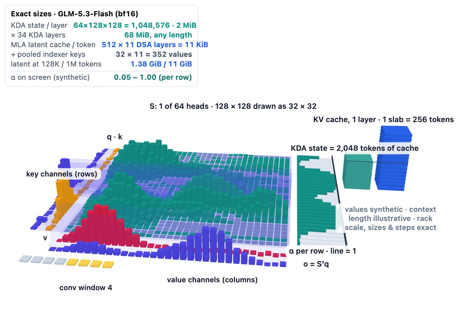
Worked numbers for one Flash KDA layer (derived from the shapes):

• Compute. Each step touches all 16,384 state entries once (three of the four as multiply-adds), so one head costs about 115K FLOPs and 64 heads about 7.3 MFLOPs per token. The projections around the core add about 275 MFLOPs. Neither depends on how long the context is.

• Memory. The state is 64 × 128 × 128 = 1,048,576 values: 2 MiB in bf16, or 4 MiB in fp32, the precision fla’s decode kernel keeps the state in while it works on it. The convolution needs the last three tokens’ 24,576 q

  k

  v channels, another 73,728 values.

• Comparison. One KDA state is as large as one Flash MLA layer’s cache of 2,048 tokens (512 values per token); at 1,048,576 tokens that MLA cache is 512 times larger (notes below).

Across 34 layers the state is 68 MiB in bf16 per sequence; §9.3 sets this against the DSA layers’ caches. Those layers are sparse, so their attention core stays bounded by 2,048 selected tokens, but they keep the full latent cache and their indexer still scores every 4-token block of the context (§8.5).

Implementation notes

• fla’s decode kernel (ops/kda/fused_recurrent.py) loops over tokens and keeps the state in fp32 registers: L2-normalize q and k (epsilon 1e-6), scale q, fade the state along the key axis, subtract $S^\top k$ from $v$, multiply by $\beta$, add the rank-1 write, read with q. It splits the 128 value columns into tiles of 32.
• Mode choice in fla’s layer: chunk mode whenever gradients are enabled, fused-recurrent mode for inference inputs of at most 64 tokens, otherwise the configured mode. The layer caches a convolution state and a recurrent state per layer.
• Comparison with MLA (derived): one Flash MLA layer caches 512 values per token, so one KDA state (1,048,576 values) equals 2,048 tokens of it; at 131,072 tokens the MLA cache is 64 times the KDA state. A dense MLA layer in absorbed form would spend about 131K FLOPs per context token on each generated token (64 heads × 512 dimensions, scores plus value sums), which equals KDA’s constant 7.3 MFLOPs at a context of only about 56 tokens.
• Miles is a training framework and only calls chunk_kda. The kernel and state precision that GLM-5.3-Flash is served with are not in our sources; the decode description above is fla’s reference path.

8.2.7 Why a 3:1 Hybrid with DSA

The price of a fixed-size memory is that it is lossy: 16,384 numbers per head cannot hold a million tokens verbatim. The GLM-9B ablation in §5.1 measured this risk. Even with only half the layers converted, GDN, the linear-attention layer that KDA refines, lost 11.28 RULER points at 128K, and the GLM-5 report used such gaps to argue for DSA in every layer of GLM-5. Flash goes further than that ablation (3:1 rather than 1:1), but keeps every fourth layer as DSA.

The Kimi Linear paper reaches a compatible conclusion from the other side: “Long-context retrieval remains the primary bottleneck for pure linear attention.” Its answer is to interleave whole layers, three KDA layers then one full-attention MLA layer. In its ablation, 3:1 gave the best validation perplexity (5.65), ahead of 1:1 (5.66), 7:1 (5.70), 15:1 (5.82), and all-MLA (5.77). The paper calls 3:1 “the best quality–throughput trade-off”.

Flash follows this layout: [KDA, KDA, KDA, DSA] repeated 11 times, plus one trailing KDA layer (§8.1). It also follows Kimi Linear in giving its attention layers no RoPE (§8.3). One difference stands out: Kimi Linear’s attention layers are dense MLA, while Flash’s are DSA, sparse MLA with an indexer. Only 11 of Flash’s 45 layers keep a per-token cache.

For its own model (48B total, 3B active), the paper reports at 128K a RULER score of 84.3 against 81.3 for an all-MLA baseline trained on the same 1.4T tokens, a KV cache up to 75% smaller, and at 1M context up to 6.3 times shorter time per output token than MLA (1.84 ms against 11.48 ms), a gain the paper calls theoretical and credits to larger batches. These numbers belong to Kimi Linear, not to Flash.

Z.ai has not published its reasoning, so why Flash chose 3:1 is unknown. Our reading is that the 11 DSA layers are the exact-retrieval path that the KDA layers lack. The card claims the hybrid preserves “precise long-context capabilities”; the sources we have contain no Flash long-context scores, so we cannot check that claim here.

Where the numbers come from

• Kimi Linear: hybrid design and Table 1 (training/validation perplexity: 3:1 9.23/5.65, 0:1 9.45/5.77, 1:1 9.29/5.66, 7:1 9.23/5.70, 15:1 9.34/5.82). The 3:1 model was the one used in the paper’s final experiments.
• Kimi Linear Table 5 (128K, all models trained on 1.4T tokens): RULER 84.3 vs 81.3 (MLA) and 80.5 (GDN hybrid); the paper’s average over eight long-context benchmarks is 54.5 vs 52.2 (MLA). Kimi Linear loses to MLA on LongBench V2 and Frames. §6.3 calls the 6.3× figure “a theoretical decoding speedup of up to 6.3×”, made possible by memory freed for larger batch sizes; at batch size 1 it reports 2.3× at 1M (Fig. 7b).
• “Up to 75%”: only one layer in four keeps a per-token cache. For Flash the same arithmetic gives 34 of 45 layers without a growing cache (derived).
• GDN result: GLM-5 report (arXiv 2602.15763), GLM-9B ablation; see §5.1.

8.3 NoPE: No Rotary Position Embedding in the Text Stack

A transformer has to learn token order from somewhere. GLM-5.3, like most recent models, rotates part of every query and key by an angle that depends on the token’s position (RoPE, §3.3). Flash rotates nothing, in any text layer. As far as the config and code show, its text stack has no explicit position signal at all (NoPE).

GLM-5.3 rotates only 64 of each head's 256 query/key dims with RoPE (rope_theta 8,000,000), while GLM-5.3-Flash rotates none (qk_rope_head_dim = 0, mla_use_nope = true). Our reading, not stated by Z.ai, is that Flash gets token order from causality instead: KDA's short convolution and decaying state, plus causal key selection in DSA. Open the full-size SVG.

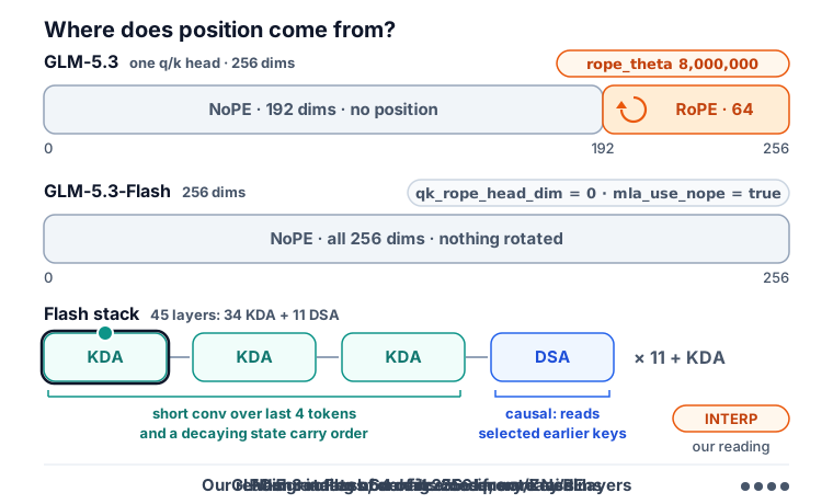
The evidence agrees across the config (qk_rope_head_dim 0, mla_use_nope true, no rope_theta or rope_parameters key) and the Miles code, whose DSA layer asserts “GLM-5.3 DSA skips rope” and whose indexer and KDA layers apply no positional encoding (notes below).

Where GLM-5.3 rotates 64 of each head’s 256 query/key dimensions (§3.3), Flash leaves all 256 position-free, and the Miles docs describe it as “NoPE MLA — multi-latent attention with the positional half of the QK head empty”.

So where does order come from? Our reading, which Z.ai does not state: from causality alone. In KDA layers the short convolution sees a window of the last four tokens, and the decaying recurrence fades older information more than newer information, so the state itself encodes recency. In DSA layers a query can only select earlier tokens. No token carries an explicit position coordinate; order shows up in which tokens are visible and how much of each survives.

Implementation notes

• Miles: miles_plugins/models/glm5_next/dsa.py asserts config.qk_pos_emb_head_dim == 0 (“GLM-5.3 DSA skips rope”) and rotary_pos_emb is None in the forward pass. The indexer code in the same file applies no rope to index_q or index_k.
• Open discrepancy, so we quote no rotary base for Flash: the Miles doc says “rotary base 800000”, the training script passes --rotary-base 10000, and the config has no rotary-base key (no rope_theta / rope_parameters). With zero rotary dimensions the value has no effect in Miles.
• The config also carries indexer_rope_interleave: true, yet Miles applies no rope in the Flash indexer. Whether a reference inference engine does is unknown from our sources; the key may be a leftover from GLM-5’s config.
• max_position_embeddings is still 1,048,576, the same as GLM-5.3.

8.4 MLA in Flash: A 512-Number Cache per Layer

The 11 DSA layers still use MLA (§3) to keep their cache small. Because Flash drops the rotary part, the per-token cache in each of these layers is just the 512-number latent, with no extra 64-number position slice.

The shapes differ from GLM-5.3 in three places:

	GLM-5.3	GLM-5.3-Flash
Heads	64	64
Query compression rank (q_lora_rank)	2,048	1,536
Key/value latent (kv_lora_rank)	512	512
Query/key dims per head	192 position-free + 64 RoPE	256 position-free
Value dims per head	256	256
Cached values per token per layer	512 + 64 = 576	512

For scale: uncompressed multi-head attention with these head sizes would cache 64 × (256 + 256) = 32,768 values per token per layer, so Flash’s MLA cache is 64 times smaller (derived). Across the 11 DSA layers that is 5,632 values per token; §9 compares this with GLM-5.3 and adds the indexer keys.

Miles runs the attention in MLA’s absorbed form (§3.4). All 64 heads attend to the same 512-number latent per token, which serves as both key and value. Afterwards a per-head matrix lifts each result from 512 back to 256 dimensions, and the output projection maps 64 × 256 = 16,384 values back to 4,096. Switch the MLA 3D model in §3.4 to Flash mode to compare the two cache entries.

Implementation notes

• Source: miles_plugins/models/glm5_next/dsa.py, a subclass of GLM-5’s DSAMLASelfAttention. Training-script flags: --q-lora-rank 1536 --kv-lora-rank 512 --qk-head-dim 256 --qk-pos-emb-head-dim 0 --v-head-dim 256.
• Absorption: linear_kv_up_proj.weight is split into w_kc and w_vc, each [64, 256, 512]. The query is einsum(q, w_kc) → [T, 64, 512]; the key is the shared 512-d latent (one KV group).
• Padding: _SPARSE_MLA_TAIL_DIM = 64 zero dims on query and key. GLM-5’s tilelang SparseMLA kernel expects 576-wide keys (512 latent + 64 rotary), so the padding lets Miles reuse it; the padded slice adds nothing to any dot product. Our reading is that this is a shortcut to avoid writing a dedicated 512-wide kernel.
• softmax_scale = q_head_dim ** -0.5 with q_head_dim = 256. The softmax scale follows the real head size rather than the padded width: $1/\sqrt{256} = 0.0625$, not $1/\sqrt{576} \approx 0.042$. In plain terms, attention logits are divided by 16 before the softmax.
• The q and kv RMSNorms are fused into linear_q_up_proj / linear_kv_up_proj, so the layer spec shows them as identity ops.
• By our count one Flash MLA block has about 117.4M parameters, plus about 7.5M for its indexer (derived).

8.5 The kpool indexer: choosing among blocks of four

Flash’s 11 DSA layers still use a lightning indexer to decide which 2,048 past tokens each query reads, with the same 32 heads × 128 dimensions and top-2,048 budget as GLM-5.3. The difference is what the indexer scores. Instead of one index key per past token, Flash first squeezes every block of 4 consecutive tokens into one pooled key (hence “kpool”, after the config key index_kpool), then picks whole blocks.

Everything else in the DSA layer is the GLM-5.3 design from §5.3: one selection list per query token, shared by all 64 heads, over MLA’s latent cache, which in Flash is the 512-number latent alone (§8.4). The index queries and head weights are also built as in §5.2, from Flash’s 1,536-wide compressed query and 4,096-wide hidden state.

The recipe, as implemented in Miles, runs in four steps:

1. Pool the keys. Each sequence is cut into non-overlapping blocks (“pools”) of 4 consecutive tokens. Every token still gets its 128-dimensional index key, and the four keys of a pool are blended into one.
2. Score complete pools only. For a query at position $t$, only pools whose 4 tokens all lie at or before $t$ are eligible. Each gets one indexer score, using the same ReLU scorer as GLM-5.3 (§5.2).
3. Pick 512 pools, expand to 2,048 tokens. The top $2{,}048 / 4 = 512$ pools win, and each expands back to its 4 token positions.
4. Always add the tail. The tokens of the current, still-incomplete pool (0 to 3 of them, including the query itself) are appended after the top-k, so the newest 0 to 3 tokens are never dropped.

There is one shortcut: a token among the first 2,048 positions of its sequence simply attends to every token up to and including itself. That is exact dense causal attention, with no indexer decision at all. GLM-5.3 reaches the same result implicitly (§5.3); Flash’s code checks for it explicitly.

Step 1 in detail. The blending is a learned, per-channel softmax. For a pool $p$ covering tokens $s, \dots, s+3$ and each of the 128 channels $d$:

\[\pi_{r,d} = \frac{\exp\left(g_{s+r,d} + a_{r,d}\right)}{\sum_{r'=0}^{3} \exp\left(g_{s+r',d} + a_{r',d}\right)}, \qquad \bar{k}_{p,d} = \sum_{r=0}^{3} \pi_{r,d}\, k_{s+r,d}\]

Here $k_{s+r}$ is a token’s index key, $g_{s+r} = W_{\text{gate}} x_{s+r}$ is a 128-dimensional gate computed from its hidden state, and $a_{r}$ is a learned bias for slot $r$ (0 to 3) inside the pool. The pool score then reuses the familiar indexer formula:

\[I_{t,p} = \sum_{j=1}^{32} w_{t,j}\, \mathrm{ReLU}\left(q_{t,j} \cdot \bar{k}_p\right)\]

In plain terms (illustrative numbers): in a pool holding “the”, “capital”, “of”, “France”, channel 7 of the pooled key might take 70% of its value from “France” and only a few percent from “the”, while channel 8 may weigh them quite differently. The slot bias $a_r$ lets the model prefer, say, the last token of each block. Each query then compares itself against one key per block instead of four.

Because each channel has its own softmax, the pooled key is not the key of any single token. It is a per-dimension mixture, so one pooled key can carry the strongest features of several tokens at once. That is our reading of why the blend is learned rather than a plain average.

Steps 2 to 4, a worked example. Take the query at position 10,001 (counting from 0), so 10,002 tokens are visible:

• Complete pools: $\lfloor 10{,}002 / 4 \rfloor$ = 2,500 eligible pools, covering positions 0 to 9,999.
• The indexer scores those 2,500 pooled keys (instead of 10,002 token keys) and keeps the top 512.
• The 512 pools expand to 2,048 token positions.
• The tail is positions 10,000 and 10,001 ($10{,}002 \bmod 4 = 2$ tokens), appended after them.

The attention kernel then reads 2,050 latent rows. Had the query been at position 10,003, the last pool would be complete, the tail empty, and that pool would compete for selection like any other.

Implementation notes

• Config keys: index_kpool 4, index_kpool_compress true, index_kpool_always_select_tail true, plus the familiar index_n_heads 32, index_head_dim 128, index_topk 2048. Miles asserts index_kpool > 1 and that both flags are true (glm5_next.py), and has no code path for turning them off; the tail is always appended (no code reads the flag).
• New weights per DSA layer: index_kpool_compress_gate [128, 4096] (the gate $W_{\text{gate}}$) and index_kpool_compress_ape [4, 128] (the slot bias $a$), stored in fp32 (dsa.py). Miles initializes both to zeros and marks them frozen, so their values must come from the checkpoint.
• Pooling and selection live in miles_plugins/models/glm5_next/ops/kpool_indexer.py: pool_boundaries cuts each sequence into $\lfloor \text{len}/4 \rfloor$ pools, _pooled_keys_kernel computes $\bar{k}$ (max-subtracted softmax in fp32), and kpool_select_topk takes min(index_topk // kpool, num_pools) = 512 pools. Scoring reuses GLM-5’s TileLang indexer kernel; ineligible pools get $-\infty$, and chosen pools with a non-finite score become index −1.
• Top-k is torch.topk on fp32 scores here, with no FlashInfer option, so the operator is the deterministic one the GLM-5 report recommends for RL (§5.7), unless the optional indexer replay supplies recorded choices (§10).
• The output index list is padded to a multiple of 64: $\lceil (2{,}048 + 3)/64 \rceil \times 64 = 2{,}112$ slots, with the tail in slots 2,048 to 2,050, so a query reads at most 2,051 real keys.
• The index key is a LayerNorm of wk(x), and the head weights $w_{t,j}$ come from weights_proj(x) in fp32, scaled by $32^{-1/2} \cdot 128^{-1/2}$. The index query is wq_b (1,536 → 32 × 128) applied to the RMS-normalized, detached compressed query.

What does this buy? Our reading of the code, not a figure Z.ai states:

• Fewer keys to score. Each indexer pass scores about $L/4$ pooled keys instead of $L$ token keys: 32 × 128 × $L$/4 = 1,024 multiply-adds per past token instead of 4,096. The pooling itself adds a fixed cost per token (the gate is a 4,096 → 128 projection), independent of $L$.
• A later crossover. Flash’s sparse attention costs about 134M multiply-adds per query token per layer. Indexer scoring catches up with it near 131K tokens, against roughly 35K for GLM-5.3’s per-token indexer (§5.3; both derived).
• Smaller index-key cache. One 128-value key per 4 tokens is 32 values per token per DSA layer, a quarter of GLM-5.3’s 128.
• Block-shaped reads. Selected keys arrive in contiguous runs of 4 tokens, a layout that is friendlier to sparse-attention kernels than 2,048 scattered positions.
• The same reading budget. The expensive MLA attention still reads 2,048 selected tokens (plus up to 3 tail tokens), exactly as in GLM-5.3.

The price, by our reading, is granularity: the indexer can no longer pick one token without its three neighbors, so part of the 2,048-token budget goes to tokens that ride along with a strong neighbor. The sources report no ablation of this trade-off, nor why the pool size is 4.

Flash does not use IndexShare: all 45 entries of its indexer_types are "full", and each of the 11 DSA layers runs its own indexer. By our reading it hardly needs sharing. Its layout already reaches the one-in-four indexer density that GLM-5.3 gets by reuse (§1.3), and pooling cuts each pass to a quarter. §9.4 puts numbers on the combined effect.

Flash’s indexer also has no position signal of its own. GLM-5.3 rotates half of each index vector with RoPE (§5.2); Flash rotates none (§8.3). Within a pool, the slot bias $a_r$ is the only positional input, and across pools the causal window is.

The Flash mode of the indexer 3D model in §5.2 covers this pool-then-expand selection, and so does the indexer animation there. The attention landscape in §5.6 also has a Flash mode for the whole 45-layer stack.

Where the numbers come from

• Indexer density: GLM-5.3 keeps an indexer on layers 0, 1, 2 and every 4th layer from 6 to 74 (21 of 78, see §5.6); Flash’s DSA layers are 3, 7, …, 43 (11 of 45, layer_types). Indexer weights exist only on those 11 layers plus the MTP layer 45, so the "full" entries for KDA layers are placeholders by our reading.
• A rough indexer-work ratio (derived, not a published number): against a model of the same depth that runs a plain per-token indexer in every layer, GLM-5.3’s indexer work is $21/78 \approx 0.27\times$ and Flash’s about $11/45 \times 1/4 \approx 0.06\times$, assuming equal cost per head and ignoring the MTP layer and pooling overhead.
• Cost figures (derived): Flash sparse attention ≈ 64 heads × (512 + 512) × 2,051 ≈ 134.4M multiply-adds per query token per layer (the kernel actually computes on 576-wide padded keys and 2,112 slots, about 147M); 134.4M / 1,024 ≈ 131K tokens. Fixed indexer projections per token: wq_b + wk + weights_proj + gate ≈ 7.47M multiply-adds.
• In Miles RL the Flash indexer is not trained: its inputs are detached, scoring runs under torch.no_grad, and the two kpool tensors have requires_grad set to False. kpool selection also raises NotImplementedError under context parallelism. §10 has more on training.
• The config sets indexer_rope_interleave true, yet Miles applies no rotary embedding to the Flash indexer’s queries or keys (§8.3). We cannot tell from local sources what the reference inference code does.

8.6 mHC: four residual lanes instead of one

In GLM-5.3, as in most transformers, every sublayer reads one residual stream and adds its output back to it. Flash widens that stream into 4 parallel lanes. Each sublayer reads a weighted blend of the lanes, writes its output back across them, and the lanes are mixed by a small 4 × 4 matrix that is constrained so the mixing cannot amplify the signal. This is the mHC technique the model card names (quoted at the start of §8).

What the config and code pin down:

• Four lanes. hc_mult 4 becomes Megatron’s num_residual_streams = 4.

• Two sites per layer. One hyper-connection wraps the attention sublayer and one wraps the FFN sublayer in every one of the 45 layers, which makes 90 mHC sites.

• A plain average at the end. Before the final norm and LM head, the 4 lanes are averaged with no learned weights.

The equations below follow the mHC paper (arXiv 2512.24880). They are our reading of how these tensors are used: the actual math lives in a Megatron-LM module (radixark/Megatron-LM#89) that we did not inspect. With the residual state $x_l$ holding 4 lanes of 4,096 values each, one site computes

\[x_{l+1} = H^{\text{res}}_l\, x_l + \left(H^{\text{post}}_l\right)^{\top} \mathcal{F}\left(H^{\text{pre}}_l\, x_l\right)\]

where $\mathcal{F}$ is the attention or FFN sublayer, $H^{\text{pre}}$ (1 × 4) blends the lanes into a single 4,096-wide sublayer input, $H^{\text{post}}$ (1 × 4) spreads the output back over the lanes, and $H^{\text{res}}$ (4 × 4) mixes the lanes with each other. All three are computed per token from the state itself, scaled by the matching $\alpha$ and shifted by the bias.

GLM-5.3-Flash replaces the single residual stream with four lanes (hc_mult = 4): at each of its 90 attention/FFN sites, 20 Sinkhorn iterations push the 4×4 mixing matrix H_res toward rows and columns that each sum to 1, and at the end the lanes are averaged. The settings are from the config and Miles code, the equations follow the mHC paper (arXiv 2512.24880), and the matrix values are illustrative. Open the full-size SVG.

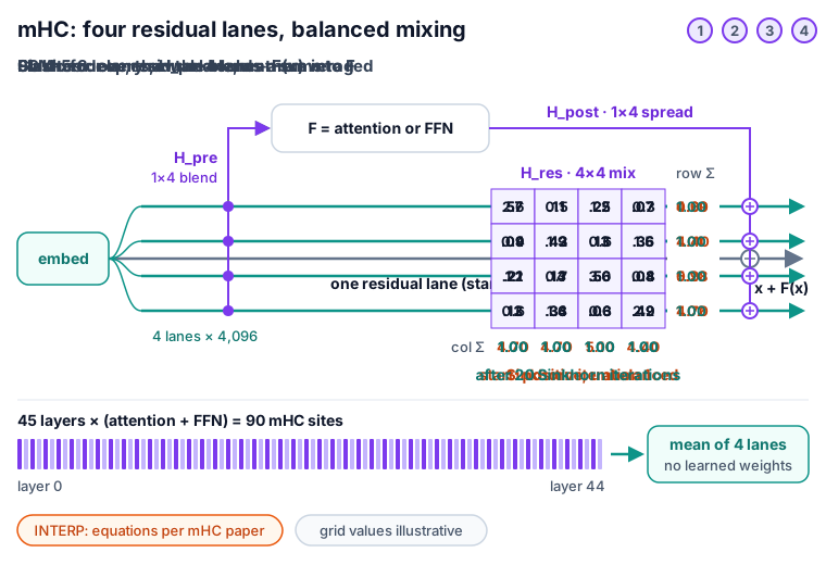
In the paper’s formulation, the constraint sits on $H^{\text{res}}$. Its raw entries are made positive with $\exp(\cdot)$, then 20 Sinkhorn iterations alternately rescale rows and columns until each row and each column sums to 1. The result is (approximately) a doubly stochastic matrix.

In plain terms: with a mixing matrix whose first row is $[0.7, 0.1, 0.1, 0.1]$, new lane 1 is 70% of old lane 1 plus 10% of each of the others. Because every column also sums to 1, each old lane hands out exactly its full weight, no more. The mHC paper’s argument is that such matrices never amplify the signal (spectral norm at most 1) and that a product of them is again doubly stochastic, so stacking 90 sites cannot make the residual path blow up or vanish.

mHC is cheap in parameters. By our count, assuming the mapping weight has the shape the paper’s formulation implies, each site holds about 0.39M weights and all 90 sites about 35M, roughly 0.01% of the model. The card says mHC is there “to further improve scaling efficiency”; by the paper’s argument, the gain is a more stable signal through 45 layers, not capacity.

A more likely cost is width: if the 4 lanes are carried between layers as the formulation implies, the hidden state passed from layer to layer is 4 × 4,096 = 16,384 values per token instead of 4,096 (our reading; we have no measurement of its memory or speed impact).

Implementation notes

• Three tensors per site. hc_{attn,ffn}_fn is a linear map that produces the mixing coefficients from the current state, hc_{attn,ffn}_base is a static bias added to them, and hc_{attn,ffn}_scale holds three scalars $[\alpha_{\text{pre}}, \alpha_{\text{post}}, \alpha_{\text{res}}]$.
• Sinkhorn with 20 iterations, hc_sinkhorn_iters 20, with hc_eps 1e-6.
• Miles maps the config to Megatron with enable_hyper_connections=True, num_residual_streams=4, mhc_sinkhorn_iterations=20, and use_fused_mhc=False (miles_plugins/models/glm5_next/glm5_next.py). It asserts hc_eps == 1e-6 because Megatron hard-codes that epsilon for Sinkhorn and for computing $H$.
• The weight bridge maps hc_*_fn to mapping_proj.weight and hc_*_base to its bias, and splits hc_*_scale into $\alpha_{\text{pre}}, \alpha_{\text{post}}, \alpha_{\text{res}}$ (slices 0, 1, 2). All hc_* tensors stay unquantized in the FP8 checkpoint.
• Miles patches the projection used to compute the coefficients: it returns $x W^{\top}$ together with a separate RMS factor $1/\sqrt{\mathrm{mean}(x^2) + \epsilon}$, with $\epsilon = 10^{-5}$ (the RMSNorm epsilon). Our reading is that this folds an RMSNorm of the flattened 4-lane state into the coefficients.
• The final contraction is Glm5NextMeanOutputContraction, described in the code as a “plain mean over the residual streams, with no learned head weights”.
• The 0.39M-per-site figure assumes hc_*_fn is $[n^2 + 2n,\ n \cdot 4{,}096] = [24, 16{,}384]$ for $n = 4$: 16 entries for $H^{\text{res}}$ plus 4 each for $H^{\text{pre}}$ and $H^{\text{post}}$. The exact shape is not verified from local sources.

8.7 MoE in Flash: 288 experts, 8 at a time

Flash’s feed-forward side follows the same recipe as GLM-5.3’s (§4), scaled to a narrower model with 288 routed experts per MoE layer instead of 256.

	GLM-5.3	GLM-5.3-Flash
Hidden size	6,144	4,096
Routed / shared experts per MoE layer	256 / 1	288 / 1
Experts per token	8 routed + 1 shared	8 routed + 1 shared
Expert FFN width (moe_intermediate_size)	2,048	2,048
Weights per expert (derived)	37.75M	25.17M
Dense layers / MoE layers	3 / 75	3 / 42
Router	sigmoid, noaux_tc, scaling 2.5, fp32	sigmoid, noaux_tc, scaling 2.5, fp32

Each expert is a SwiGLU block of three 4,096 × 2,048 matrices. The 3D expert-city model in §4 has a Flash toggle that shows the 288-expert grid.

Two config keys are new relative to GLM-5.3’s config, which has neither:

• A small auxiliary balance loss. router_aux_loss_coef 0.001. Load balancing presumably still relies mainly on the selection-only expert bias of noaux_tc (§4); the coefficient adds a light loss-based nudge on top. How it is applied in pre-training is not described in the sources.
• An activation clamp. swiglu_limit 10. Miles passes it to Megatron as --activation-func-clamp-value 10, with a code comment that the checkpoint’s limit is one “which sglang applies to dense, shared and routed MLPs”. The vision tower’s config carries the same limit.

The experts dominate the parameter count even more than in the flagship. By our count the routed experts hold 304.4B weights, 97.2% of the 313.3B text parameters, and a token touches about 226.5M of the roughly 7.27B weights in each MoE layer (about 3%). §8.9 reconciles these counts with the card’s 320B total and 18B active.

Implementation notes

• Miles’ Megatron arguments: --num-experts 288, --moe-router-topk 8, --moe-ffn-hidden-size 2048, --moe-shared-expert-intermediate-size 2048, --moe-router-score-function sigmoid, --moe-router-enable-expert-bias, --moe-router-topk-scaling-factor 2.5, --moe-router-dtype fp32, and --moe-layer-freq = [0]*3 + [1]*42.
• Config: n_group 1, topk_group 1 (no group-limited routing), norm_topk_prob true. The per-layer expert bias is stored as mlp.gate.e_score_correction_bias.
• In Miles RL, --moe-router-bias-update-rate 0 freezes that bias, and --enable-r3 turns on rollout routing replay (§10).
• The exact form of the clamp (which of the gate and up projections are clamped, and how) lives in SGLang and Megatron code we did not inspect.

8.8 Native vision: a 24-layer ViT in front of the text stack

GLM-5.3 reads text only; Flash also reads images and video (§1.1). The mechanism is the familiar one: a vision encoder, here a ViT, turns pixels into vectors of the text model’s width, and those vectors sit in the token sequence like ordinary tokens.

The vision_config describes a small encoder next to the 4,096-wide text stack:

Field	Value
Transformer blocks (depth)	24
Hidden size / heads	1,024 / 16 (head dim 64, derived)
MLP width	4,096 (SiLU)
Patch size / default image size	14 px / 448 px
Temporal patch / spatial merge	2 frames / 2 × 2 patches
Output width (out_hidden_size)	4,096 (= text hidden size)
Projector MLP width	10,240
Activation clamp (swiglu_limit)	10

In plain terms (derived, assuming the merge works as in earlier GLM-V models): a 448 × 448 image cuts into $32 \times 32 = 1{,}024$ patches of 14 × 14 pixels. Merging each 2 × 2 group leaves 256 vectors, each projected to 4,096 values, so the image enters the text model as 256 tokens. For video, the temporal patch of 2 groups pairs of consecutive frames into one patch.

The encoder is tiny next to the language model. By our count it holds about 0.56B weights, under 0.2% of the 320B total; this assumes a module layout like the GLM-4.xV encoders, whose module names match the names listed in Flash’s checkpoint config exactly.

Implementation notes

• Module names visible in the FP8 skip-list: visual.patch_embed.proj, visual.blocks.{0..23} (with attn.qkv, attn.q_norm, attn.k_norm, attn.proj, and SwiGLU mlp.gate_proj / up_proj / down_proj), visual.post_layernorm, visual.downsample, and visual.merger.*. All visual.* weights stay in BF16 in the FP8 checkpoint.
• Special tokens: image_token_id 154854 and video_token_id 154855 mark images and videos; boundary tokens are image start/end 154830/154831 and video start/end 154832/154833. The card’s pipeline tag is image-text-to-text, and its benchmark footnotes include the vision benchmark BabyVision.
• Our 0.56B splits as 24 blocks (403.0M), merger (142.6M), downsample (16.8M), and patch embedding (1.2M). Any vision position embedding is not modelled.
• Miles’ Flash support is text-only for now: its chat-template code notes that “Flash support covers tokenizer text inputs, not multimodal processor inputs.”

8.9 Reconciling the parameter count

The card says Flash has “320B total parameters and just 18B active parameters”. Neither number appears in the config, so we recounted from the config and the Miles code. The totals land close to the card, but only under a counting convention that differs from the one that reproduces the flagship’s 744B.

Component (derived)	Total	Active per text token
Text stack: 45 layers + embeddings + LM head	313.33B	17.38B
MTP layer 45 (shares embeddings and LM head)	7.43B	0.39B, if counted
Vision tower	0.56B	0, unless the token is an image token
Sum	321.32B	17.38B to 17.94B
Card	320B	18B

Where the numbers come from

• Total. Our 321.3B matches “320B” within about 0.4%, but only when the MTP layer and the vision tower are both counted. Text alone is 313.3B, and text plus vision without MTP is 313.9B.
• Active. 17.38B for the 45 main layers (with embeddings and LM head), 17.76B with the MTP layer, and 17.94B with the vision tower as well. Embeddings and LM head are counted here, unlike the GLM-5 report’s convention in §2.3. The last two figures round to the card’s 18B; the main-stack figure is about 3.5% below it. Which count Z.ai means is not stated.
• All counts come from a script over config.json (params_flash.py in our fact base). KDA shapes come from Miles kda.py, DSA attention from the GLM-5 MLA layout with qk_rope_head_dim 0, indexer and kpool tensors from dsa.py, and MoE sizes from the config.
• Assumed shapes: the mHC mapping weight (about 0.04B in total) and the vision layout (about 0.56B). Together they account for only about 0.6B of the total.
• Text-stack breakdown: routed experts 304.41B, KDA attention 4.68B (34 layers), DSA MLA 1.29B and indexers 0.08B (11 layers), shared experts 1.06B, embeddings and LM head 0.63B each, dense FFN 0.45B, routers 0.05B, norms and mHC 0.04B.
• Excluding the embedding table, active weights are 16.74B; excluding both the embedding table and the LM head, 16.11B.

9. Memory and Compute Arithmetic, Side by Side

How much memory does each model need to hold a very long conversation, and how much work does each new token cost? The short answer: both models cap the attention work per token, but GLM-5.3-Flash also stops most of its layers from keeping a per-token cache, so its memory grows about 8× more slowly with context.

Everything in this section is derived by us from the two config.json files (and, for compute, the official active-parameter counts). It is back-of-envelope arithmetic for one sequence in bf16 (2 bytes per value), not a measurement. Our sources contain no measured serving-memory or speed numbers for either model.

44,928GLM-5.3 cached values per token78 layers × (512 + 64), derived

5,632Flash cached values per token11 DSA layers × 512, derived

~8×smaller growing cache44,928 / 5,632 = 7.98, derived

68 MiBFlash KDA statebf16; fixed per sequence, any length

9.1 The growing cache: what each new token adds

A cache that grows with context is the main memory cost of long conversations. Every layer that does softmax attention must keep something for each past token so later queries can look back at it.

• GLM-5.3. All 78 layers are MLA layers. Each stores the 512-value latent plus the 64-value RoPE key, so one token adds $78 \times (512 + 64) = 44{,}928$ values. That is 89,856 bytes, about 88 KiB, in bf16.
• GLM-5.3-Flash. Only the 11 DSA layers keep a per-token cache, and their MLA is NoPE, so there is no RoPE part: $11 \times 512 = 5{,}632$ values, or 11,264 bytes (11 KiB). The 34 KDA layers add nothing per token.
• Flash’s pooled indexer keys. The kpool indexer keeps one 128-value key per group of 4 tokens, which is 32 values per token per DSA layer, or $11 \times 32 = 352$ more. With them, Flash adds 5,984 values (11,968 bytes) per token.

In plain terms: for every token you append, GLM-5.3 writes about 88 KiB into its cache and Flash about 11 KiB, or about 12 KiB counting the pooled indexer keys. The ratio is 7.98×, or about 7.5× with Flash’s pooled keys included.

9.2 At one million tokens

Multiply by the context length. Both configs allow 1,048,576 positions; the table also shows a round $10^6$ tokens, since “1M” is often read that way.

Per sequence, bf16 (derived)	GLM-5.3	GLM-5.3-Flash
Growing cache at $10^6$ tokens	44.9G values, ~90 GB	5.6G values, ~11.3 GB (~12.0 GB with pooled keys)
Growing cache at 1,048,576 tokens	87.75 GiB (~94 GB)	11 GiB (~11.8 GB); 11.7 GiB with pooled keys
Fixed state, independent of length	none	68 MiB of KDA state (+ ~5 MiB conv state)

These are orders of magnitude, not serving numbers. The gap comes from two choices at once: Flash keeps a per-token cache in 11 layers instead of 78, and its NoPE MLA drops the 64 RoPE values from each entry.

9.3 The fixed-size notebook: Flash’s KDA state

The 34 KDA layers trade the growing cache for a constant one. This is where the animation in §8.2 ends up: each head keeps one 128 × 128 matrix that is updated in place as tokens arrive.

\[34 \text{ layers} \times 64 \text{ heads} \times 128 \times 128 = 35{,}651{,}584 \text{ values} \approx 68 \text{ MiB (bf16)}\]

In plain terms: Flash’s KDA memory is the same 68 MiB whether the conversation is 10 tokens or 1,000,000 tokens long. It equals the DSA cache of about 6,300 tokens ($35{,}651{,}584 / 5{,}632 \approx 6{,}330$). Past that point the growing cache dominates, and at 1,048,576 tokens the KDA state is about 0.6% of Flash’s total.

Where the numbers come from

• GLM-5.3: num_hidden_layers 78, kv_lora_rank 512, qk_rope_head_dim 64. MLA caches the compressed latent plus the shared RoPE key; the GLM-5 report describes MLA decoding as a 576-dimensional dot product (512 + 64).
• Flash: 11 layers of type deepseek_sparse_attention, kv_lora_rank 512, qk_rope_head_dim 0 (mla_use_nope true). KDA: linear_attn_config with 64 heads × head_dim 128 and short_conv_kernel_size 4.
• Pooled indexer keys: index_head_dim 128, index_kpool 4. Without pooling, the Flash indexer keys would be $11 \times 128 = 1{,}408$ values per token.
• Conv state: the short convolution runs over q, k and v (3 × 8,192 channels) and needs the previous 3 inputs, so about $34 \times 24{,}576 \times 3 \approx 2.5$M values, or ~5 MiB. Our reading of the kernel size; not stated as a cache size anywhere.
• Not counted: the MTP layer, and the GLM-5.3 indexer keys. If each of the 21 full-indexer layers cached one 128-value key per token, that would add 2,688 values per token (derived; the cache format is not in our sources). The ratio stays near 8× either way: 47,616 vs 5,984 values is 7.96×.
• Precision: everything is bf16 (although fla’s reference decode kernel keeps the KDA state in fp32, 136 MiB across 34 layers; the serving precision is not in our sources). Miles’ GLM-5.2 rollout recipe uses an fp8_e4m3 KV cache in SGLang; storing one byte per value would roughly halve these figures before scale factors. We did not compute FP8 layouts.
• Units: GB = $10^9$ bytes, GiB = $2^{30}$ bytes.

9.4 Compute per token: what still grows with context

Caching is only half the story; each new token also costs arithmetic. In both models the expensive softmax attention is capped, so the one piece that still grows with context is the lightning indexer, which scores every earlier key (or, in Flash, every earlier pool of 4 keys).

• Sparse attention. Each DSA layer attends to at most 2,048 selected tokens, however long the context. Flash adds the 0 to 3 tokens of the current incomplete pool, so at most 2,051.
• KDA. Each KDA layer does a fixed number of 128 × 128 matrix operations per head per token, independent of context.
• Indexer. GLM-5.3 runs an indexer in 21 of 78 layers, each scoring all $L$ earlier keys. Flash runs one in 11 of 45 layers, each scoring $L/4$ pooled keys. Per token, that is $21L$ versus $11 \times L/4 = 2.75L$ key scores, about 7.6× fewer for Flash.

To see the sizes, here is a rough per-token count at a context of $10^6$ tokens. It counts FLOPs (1 GFLOP = $10^9$) using the rule of thumb of 2 FLOPs per active parameter for the weight matrices, plus the attention and indexer terms above.

Per token at $10^6$ context, derived	GLM-5 / 5.1 (indexer every layer)	GLM-5.3	GLM-5.3-Flash
Weight matmuls ($2 \times$ active params)	~80 GFLOPs	~80 GFLOPs	~36 GFLOPs
Sparse attention over ≤ 2,048 keys	~22 GFLOPs	~22 GFLOPs	~3 GFLOPs
Indexer scoring	~639 GFLOPs	~172 GFLOPs	~22.5 GFLOPs
Rough total	~741 GFLOPs	~274 GFLOPs	~62 GFLOPs

In plain terms: at a million tokens of context, the indexer dominates GLM-5’s per-token arithmetic, IndexShare cuts that term by 3.7×, and Flash’s fewer, pooled indexer layers cut it by a further 7.6×. Our GLM-5 to GLM-5.3 ratio of about 2.7× is in the same range as the GLM-5.2 card’s “2.9x” per-token FLOPs claim at 1M context, though the card does not state its baseline or counting method.

Where the numbers come from

• Active parameters: 40B for GLM-5.3 (it shares GLM-5.2’s base, 744B / 40B) and 18B for Flash (its card). FLOPs ≈ 2 × active parameters is a standard estimate that ignores norms, routing, mHC mixing and the MTP layer.
• Indexer: index_n_heads 32 × index_head_dim 128 in both models. Each key score is a 32-head dot product against one 128-value key: $32 \times 128 = 4{,}096$ multiply-adds, or 8,192 FLOPs. GLM-5.3: $21 \times 10^6 \times 8{,}192 \approx 172$ GFLOPs. Flash: $11 \times 250{,}000 \times 8{,}192 \approx 22.5$ GFLOPs. GLM-5 / 5.1 (all 78 layers): $\approx 639$ GFLOPs.
• Sparse attention: absorbed MLA scores the query against each selected 576-value entry (512 + 64) and then sums 512-value latents, per head. GLM-5.3: $2{,}048 \times 64 \times (576 + 512) \times 2 \times 78 \approx 22.2$ GFLOPs. Flash (no RoPE part; its kernel zero-pads to 576 width): $2{,}051 \times 64 \times (512 + 512) \times 2 \times 11 \approx 3.0$ GFLOPs.
• KDA: a few 128 × 128 operations per head per layer: about 7.3 MFLOPs for the recurrent core plus 275 MFLOPs for the projections per layer and token, independent of context length (derived, §8.2.6).
• FLOPs are not time. Decoding is often limited by memory traffic, so the cache sizes in §9.1 and §9.2 matter as much as this table. None of these numbers are measurements.

9.5 What the cards claim, and what this arithmetic does not show

The arithmetic matches the direction of the Flash card, which says the hybrid design is “sharply reducing long-context serving costs while preserving precise long-context capabilities”. The card also says Flash “outperforms GLM-5.2 across benchmarks and real-world workloads at one-tenth the price”. It does not give the basis for that price comparison, and its benchmark results appear only as an image.

Of the two routes to a similar indexer budget (§1.3), only Flash also shrinks the growing cache.

10. Training notes from the open implementation (Miles)

Z.ai has not published a training recipe for GLM-5.3 or GLM-5.3-Flash (the GLM-5 report names its slime framework for GLM-5). The open RL framework Miles, covered in our earlier deep dive, has added GLM-5.3-Flash support, and that code is the best public view of what it takes to run the new hybrid in a training loop. This section collects what it shows. It describes how Miles post-trains Flash with RL; it is not Z.ai’s own recipe.

10.1 The setup

Flash support landed in radixark/miles#2786, paired with the SGLang branch sglang-miles-glm53next and radixark/Megatron-LM#89. The recipe lives in docs/models/glm/glm5-3-flash.md in the Miles repository. Two choices stand out before any numbers:

• MTP is dropped for training. The MTP layer from §6 sits out this RL setup.
• Pipeline stages are uneven. With four pipeline stages, the 45 layers split 11 / 11 / 11 / 12, because 45 does not divide by 4.

The training recipe itself is short: GRPO (Group Relative Policy Optimization) on the DAPO-Math-17k dataset (DAPO is an RL recipe; here it is also the dataset’s name), Adam at a constant learning rate of $10^{-6}$, at most 8,192 tokens per GPU, and full recomputation of activations. Rollout is colocated with training, and the trainer is offloaded to disk. Both DSA paths run on TileLang kernels, the KV cache is BF16, and routing replay (R3) turns on with --enable-r3.

Implementation notes

The documented parallel layouts:

Cluster shape	Tensor parallel (TP)	Pipeline parallel (PP)	Expert parallel (EP)	Rollout engine
16 nodes × 4 GPUs (full model)	8	4	16	8 GPUs, SGLang TP 8 / EP 8
8 nodes × 4 GPUs (full model)	8	4	8	8 GPUs, SGLang TP 8 / EP 8
2 × 4 or 1 × 8 GPUs (4-layer slice)	2	2	2	4 GPUs, SGLang TP 4 / EP 4

• Launch: python scripts/run_glm5_3_flash.py train --model-name GLM-5.3-Flash --num-nodes 16 --num-gpus-per-node 4 --num-rollout 20 --rollout-max-response-len 4096. A smoke test uses the GLM-5.3-Flash-4layer slice with --num-nodes 1 --num-gpus-per-node 8.
• The pinned image is docker.io/radixark/miles:glm53next (GB300 and x86), which fixes the Miles, SGLang, and Megatron-LM commits together.
• The script’s docstring and the doc’s healthy-run section say “DAPO”, but the script passes --advantage-estimator grpo with an asymmetric clip of 0.2 / 0.28 and zero KL and entropy coefficients. By our reading, “DAPO” names the dataset (plus the clip-higher setting); the advantage estimator is GRPO.
• Rollout settings in the script: 4 prompts per rollout batch, 8 samples per prompt, temperature 0.8, a math reward, and one training step per rollout.

10.2 What a healthy run looks like

The Miles doc reports a validation run from #2786 on 16 nodes × 4 GB300 GPUs:

0.0068–0.0106train/rollout log-prob gapabsolute difference, first 11 rollouts

0.5 → 0.94raw rewardwithin 10 rollouts

~2.6e-4PPO KLtrain/ppo_kl

0.31–0.49gradient normtrain/grad_norm

The first card is the one to watch. The doc calls train/train_rollout_logprob_abs_diff “the one to read first on a fresh bring-up: it covers the KDA, DSA and hyper-connection paths at once.” In plain terms: SGLang and Megatron each compute the log-probability of every sampled token. If either side implements KDA, the sparse attention path, or the mHC residual mixing slightly differently, the two numbers drift apart. By our reading, a gap around 0.01 says the two engines agree closely.

10.3 What the code says about the hybrid’s moving parts

Reading the Flash model code in Miles turns up three facts that matter for anyone training it:

• The indexer is not trained in Miles RL. The lightning indexer’s inputs are detached, its scoring runs under torch.no_grad, and the kpool pooling parameters have requires_grad set to False. An optional --freeze-indexer flag also freezes the indexer’s projections. This matches the GLM-5 report’s RL default (§5.7); neither source says how Z.ai treats the indexer when training GLM-5.3 or Flash.
• Indexer choices can be replayed. Besides MoE routing replay (R3), the code has an optional indexer replay path that can reuse the top-k positions chosen during inference. Our reading: it keeps training and rollout attending to the same tokens. The GLM-5 report judged such replay impractical at $k = 2{,}048$ and used a deterministic top-k instead (§5.7).
• Context parallelism (CP) waits on the DSA layers. KDA layers already support it, but kpool selection raises NotImplementedError when CP > 1, so Flash currently trains with CP 1 and cannot split one long sequence across GPUs.

10.4 A chat-template detail that bites in RL

GLM-5.3 and GLM-5.3-Flash share a new chat-template family. Both templates start generation with <think> even when enable_thinking=False. Miles therefore pins enable_thinking=True and clear_thinking=False for this family and requires reasoning_effort to stay consistent across a session. Its agentic-rollout guide selects the matching TITO tokenizer with --tito-model glm53 (GLM-4.7, GLM-5, and GLM-5.2 use glm47). For Flash, this support covers text inputs only, not the multimodal processor.

Both model cards document the matching inference knobs. reasoning_effort takes low, high, or max and defaults to max, which the card recommends keeping for benchmark reproduction. clear_thinking defaults to false; the cards ask chat applications to pass true. Our reading: the default keeps earlier reasoning in context, which suits agent loops and keeps the token prefix append-only for multi-turn RL, while true strips it for ordinary chat.

What about GLM-5.3 itself?

Miles has no separate page for GLM-5.3 (non-Flash); its model index lists GLM-5 and GLM-5.2 as “744 B-A40B”. Because GLM-5.3’s config matches GLM-5.2’s apart from FP8 packaging, our reading is that the GLM-5.2 path in Miles applies; no source states this. That GLM-5.2 path is the 64-GPU case study in Section 9 of our Miles post. Nothing here suggests that Z.ai trained GLM-5.3 with Miles.

11. Open Questions

What could we not settle from the configs, cards, papers and Miles code? This section lists the gaps plainly so you know which claims in this post rest on our reading, not on a source.

Parameter counts and conventions

• The 744B and 320B totals. Our recounts land within about 1% of both official figures, but under opposite conventions: the flagship’s 744B (stated for the GLM-5 / GLM-5.2 base; the GLM-5.3 card gives no count) matches only without its MTP layer (§2.3), and Flash’s 320B only with its MTP layer and vision tower (§8.9). Either the two figures count differently or Flash has weights we are not modelling. The safetensors indexes would settle it, and we did not have them.

Config fields without documentation

• index_share_for_mtp_iteration is true in GLM-5.2, GLM-5.3 and Flash. The name suggests the MTP layer reuses an indexer result across draft steps, but no source says so.
• index_topk_pattern is null in GLM-5.2 and GLM-5.3. It may be a hook for an explicit sharing pattern; that is a guess.
• Flash’s indexer_types lists all 45 layers as "full", including the 34 KDA layers that have no indexer. What the entries mean for KDA layers is undocumented.

Flash’s position handling

• Rotary base and indexer RoPE. The Miles doc, the Miles script and the config disagree on a rotary base (inert with zero rotary dimensions, so we quote none), and the config sets indexer_rope_interleave true although the Miles indexer applies no rotation (§8.3 notes). Whether the reference HF or SGLang implementation applies a partial RoPE in the indexer, we could not check.

Mechanisms we described from papers, not from code

• KDA gate and mHC equations. The KDA gate formula and chunk size are read from fla at commit 8024667ab58f; Miles requires fla ≥ 0.4.2 and pins no commit, so the exact version Z.ai trained with, and the kernel used for serving, are not in our sources. The mHC weight shapes and mixing equations live in radixark/Megatron-LM#89, which we did not inspect; §8.6 follows the published mHC (arXiv:2512.24880) form, and our ~35M mHC estimate assumes a shape.

How GLM-5.2 and GLM-5.3 were trained

• IndexShare training. GLM-5.2 and GLM-5.3 ship a regular pattern (3 leading full layers, then one in every 4), close to the uniform interleaving that the IndexCache paper found loses quality when applied without training but roughly matches full DSA with its training-aware method (§5.6). For GLM-5, the paper only says the authors “plan to apply training-aware IndexCache to this production-scale model in the near future”; neither card says whether GLM-5.2 or GLM-5.3 used it.
• The 1M context. The GLM-5 report’s mid-training stops at 200K tokens; how GLM-5.2 was extended to 1,048,576 tokens (besides the rope_theta change) is not described in our sources (§6.1).
• GLM-5.3’s post-training. The card says every gain over GLM-5.2 comes from post-training, but there is no GLM-5.3 technical report. The GLM-5 recipe is lineage, not a confirmed description of GLM-5.3.

Flash’s results and price

• Benchmarks. The Flash card shows its benchmark results only as an image, and the footnote for Agents’ Last Exam is empty. We quote no Flash scores.
• “One-tenth the price.” The card does not say which prices, which tier or which date the comparison uses.

Smaller loose ends

• The GLM-5 report says the model has 80 layers; every config says 78 plus 1 MTP layer.
• The Flash MTP layer (layer 45) has DSA attention and an MoE FFN but no hc_* parameters. Our reading is that it is not wrapped in mHC; Miles drops MTP for training, so its code does not confirm this.
• GLM-5.3 ships under a custom license (other, glm-5.3) whose terms are not in our sources. GLM-5.2 and Flash are MIT.
• The GLM-5.2 card’s new_version points to zai-org/GLM-5.3-BF16, while the GLM-5.3 config we read is the FP8 one. How the BF16 and FP8 repos are named is not fully clear.

---

References

Papers

• GLM-5: from Vibe Coding to Agentic Engineering (arXiv:2602.15763) — the GLM-5 technical report: MoE, MLA, DSA, and the post-training lineage.
• IndexCache: Accelerating Sparse Attention via Cross-Layer Index Reuse (arXiv:2603.12201) — the paper the GLM-5.2 card links as IndexShare.
• mHC: Manifold-Constrained Hyper-Connections (arXiv:2512.24880) — cited for the mHC equations only.
• Kimi Linear (arXiv:2510.26692) — KDA’s origin: update rule, chunkwise algorithm, hybrid ablation and results used in §8.2.
• DeepSeek-V3 Technical Report (arXiv:2412.19437) — background: aux-loss-free (noaux_tc) bias balancing in §4.3.

Model cards and configs

• zai-org/GLM-5.3
• zai-org/GLM-5.3-Flash
• zai-org/GLM-5.2
• GLM-5.3-Flash blog (Z.ai), linked from the Flash card.

Open implementation

• radixark/miles — see docs/models/glm/glm5-3-flash.md and docs/models/glm/glm5-2.md.
• radixark/miles#2786 — GLM-5.3-Flash support in Miles.
• radixark/Megatron-LM#89 — the Megatron side, including mHC (not inspected for this post).
• flash-linear-attention — the KDA kernels Miles calls; §8.2 reads the gate, chunked and decode code at commit 8024667ab58f.

On this blog

• Miles v0.1 Deep Dive — R3, TITO, and the GLM-5.2 744B case study.