Meta released two open-weight models nine weeks apart. On August 10, 2026, it released Muse Glimmer 30B under Apache 2.0, a dense model “distilled from Muse Spark and purpose-built for autonomous agentic tasks on consumer hardware.” Its primary design constraint, according to its technical report, was to “operate reliably within a strict 32 GB VRAM envelope.” On October 15 it released Muse Spark Open under the Muse Model License: “816B total / 42B active” parameters, a 1M-token context, and a BF16 (bfloat16) checkpoint that Meta’s docs serve “on eight GPUs, such as 8 × B300.” Quantized to about 4 bits, the first fits on one consumer GPU. The second needs a multi-GPU server or, per Meta’s docs, two M5 Ultra Mac Studios with 512 GB of unified memory each.

Read the code and the two turn out to be one machine at two scales. Spark Open’s implementation in Hugging Face (HF) Transformers is written as a patch on Glimmer’s. In its modular file, 18 of the 30 classes (by our count) subclass a Muse Glimmer class, for example class MuseSparkTextAttention(MuseGlimmerTextAttention). Both models use the same grouped-query attention (GQA) with a learned sigmoid gate on its output and a weightless normalization of queries and keys (QK-norm), the same rhythm of three local, sliding-window layers per global layer, sandwich norms (a norm before and after each sublayer), a soft-capped output head (a tanh keeps every logit inside ±20), one 202,048-token vocabulary and the same vision-encoder architecture. On top of that skeleton Spark changes four things: a per-head output norm in attention, norm-preserving residual gates, a latent mixture-of-experts (MoE) layer in place of the dense feed-forward network (FFN), and an audio encoder.

The pair also gives two answers to one design question: should the feed-forward parameters be dense or split into experts? Glimmer’s report answers for the small model. Under the 32 GB ceiling, ladders of dense models (series of models of growing size trained with one recipe) were “2×-2.5×” more compute-efficient than MoE ladders with the same memory footprint, so the team “selected a dense 30B parameter design.” Spark Open gives the opposite answer: 256 experts in every layer, 816.68B decoder-block parameters stored and 42.78B used per token (derived, §2.3). This post reads Spark’s design out of its config and code, and leans on Glimmer’s report wherever the two models share a part.

Four numbers summarize what follows. All four are derived from the public configs and code; the sections in parentheses show the arithmetic.

5.24%of Spark's decoder parameters active per token42.78B of 816.68B; the official "816B / 42B" fit the 62 decoder blocks alone (our reading; §2.3)

64.4 GiBBF16 key-value (KV) cache for one 1M-token sequenceonly 16 of 62 layers keep a growing cache; 248 GiB if every layer were global (§7.2)

4,096width at which Spark's experts run, inside an 8,192-wide modelhalves every expert; the same 256 experts at full width would make a 1.61T model (§4.3)

43.78attention temperature, the fixed scale on every attention logit, in both modelsquery multiplier × √head width: 3.87 × √128 (Glimmer) = 5.473 × √64 (Spark); every attention logit lies within ±43.78 (§3.2)

This post is built from public sources, and it says which source each claim comes from:

• Model cards and configs: Spark Open’s model card (the card of the NVFP4 build, in NVIDIA’s 4-bit floating-point format), the Muse Glimmer 30B card and config, and the Hugging Face repo metadata with parameter and dtype counts. Downloading the official Spark Open weights requires accepting the Muse Model License. Spark’s config values come from the Transformers v5.20.0 code defaults and from the config.json in mlx-community’s public MLX conversion, which redistributes the model under the Muse Model License and adds only quantization keys; the two agree in every structural field the code defines (the code has no num_shared_experts).
• Code: the Transformers implementations of Muse Glimmer (added in v5.15.0) and Muse Spark (added in v5.20.0, read at that tag); llama.cpp’s graphs and converters; mlx-lm; TorchTitan’s Muse Spark implementation and recipes; and Miles’ Muse Spark Open recipe.
• Papers: the Glimmer report, “Muse Glimmer 30B: An On-Device Agentic Model” (arXiv 2610.24628, submitted October 17, 2026); and the Muse Spark Safety & Preparedness Report (arXiv 2606.12429, submitted May 14, 2026), which covers the closed Muse Spark, not Spark Open.
• Blogs and docs: Meta’s launch posts on research.meta.ai, its developer docs, the PyTorch blog, and day-0 posts from Hugging Face, vLLM and SGLang.

Where we give a reason for a shared design choice, it comes from the Glimmer report, and we say so; for the parts only Spark has, the evidence is the code and the config. Numbers come from the configs, code and cards unless we say otherwise. Numbers we computed ourselves, such as parameter breakdowns and cache sizes, are marked “derived.” Values read off a plot are marked approximate. Our readings of the evidence are marked as interpretation.

You should know what a large language model (LLM), attention and a transformer layer are. A few building blocks were explained in earlier posts, and we recap each in a sentence or two. The GLM-5.3 deep dive covers Multi-head Latent Attention (MLA, its §3), the MoE router with bias-based load balancing (its §4.3) and manifold-constrained hyper-connections (mHC, its §8.6); the DeepSeek-V4 deep dive covers sliding-window attention with sinks (its §3.4) and its MoE layers (its §8). Muse uses neither MLA nor mHC, but both are useful points of comparison.

The sections build on each other:

• §1: the family at a glance: from the closed Muse Spark to two open models, a side-by-side table, and the list of what the two share and what Spark changes.
• §2: a tour of the layers: the path of one token, the three-local-one-global schedule, and where the parameters live (3D model: the two layer stacks side by side).
• §3: attention: grouped-query shapes, the weightless QK-norm and its fixed temperature, the sigmoid output gate and Spark’s output norm, rotary position embeddings (RoPE) on local layers only, and the MLA variant Glimmer tried and dropped (3D model: one gated attention layer).
• §4: Spark’s latent MoE: the router, pooling to 4,096, the norms inside the block, what is missing, and why Glimmer is dense (3D model: the experts and the latent).
• §5: the residual stream: Glimmer’s sandwich norms, Spark’s norm-preserving residual gate, the variants of RMSNorm (root-mean-square normalization), and the normalized embeddings and soft-capped head (3D model: the residual stream on a unit circle).
• §6: perception: the shared Perception Encoder, how patches become tokens, and Spark’s convolutional audio encoder.
• §7: long context: 1M positions without RoPE scaling, the KV cache, compute per token, and fitting the weights in memory (3D model: memory and compute against context length).
• §8: speculative decoding with separate DFlash drafters instead of a built-in multi-token-prediction (MTP) head.
• §9: training: Glimmer’s co-distillation from Muse Spark, Spark Open’s safety post-training and reasoning control, and the TorchTitan and Miles recipes.

Companion Slides

A 31-slide deck covers the same ground in talk form, section by section, with the post’s figures and 3D models.

Open the deck in Google Slides.

---

1. The Family at a Glance

Where do the two open Muse models come from, and how far apart are they? This section places them on Meta’s public timeline, lines them up side by side, and sorts their parts into “shared” and “changed.” The short answer: Muse Glimmer 30B was distilled from Muse Spark; Muse Spark Open is, in Meta’s words, “the open-weight release of Muse Spark,” with extra safety post-training; and in the code the big model is written as a patch on the small one.

1.1 From Muse Spark to two open models

The family starts with a closed model. On April 8, 2026, Meta introduced Muse Spark as “the first in the Muse family of models developed by Meta Superintelligence Labs.” Three point releases followed: Muse Spark 1.1 on July 9, together with “a public preview of the new Meta Model API”; Muse Spark 1.2 on August 5, “a coding-focused update to Muse Spark 1.1,” launched with Muse Code (beta), a terminal coding agent; and Muse Spark 1.3 on September 2, “with max reasoning.”

The open weights came in two steps. On August 10, Meta released Muse Glimmer under Apache 2.0. Its model card calls it “a 30-billion-parameter causal language model with a dedicated perception encoder, distilled from Muse Spark and purpose-built for autonomous agentic tasks on consumer hardware.” On October 15 Meta released Muse Spark Open under the Muse Model License, with “816B total/42B active” parameters and a 1M-token context (model card). On October 17 the Glimmer technical report appeared on arXiv: “Muse Glimmer 30B: An On-Device Agentic Model” (2610.24628). The report explains the design choices behind Glimmer, many of which Spark shares; for Spark’s own parts, this post reads the code and the config.

Meta’s model page describes how Spark Open relates to the closed model: “Muse Spark Open is derived from the Muse Spark model we released in August, with additional safety post-training to make it more robust against misuse as a standalone model without system guardrails.”

Glimmer’s report describes its own lineage in more detail. It trains the base model “by logit distillation from Muse Spark,” “logging the top 256 logits from Muse Spark during its pre-training,” and then post-trains it with supervised fine-tuning on Muse Spark trajectories, on-policy distillation from Muse Spark and reinforcement learning (§9.1). The report states one more inheritance: Glimmer “employs the Llama 4 Byte-Pair Encoding (BPE) tokenizer with a total vocabulary of 202,048 tokens” (the “Tokenizer” subsection), and Spark Open “shares its tokenizer and vocabulary with Muse Glimmer,” according to its Transformers documentation. Beyond the tokenizer, the sources mention Llama 4 as a predecessor or a point of comparison: the Muse Spark launch post says its rebuilt pre-training stack reaches the same capabilities as “our previous model, Llama 4 Maverick” with “over an order of magnitude less compute,” and the Glimmer report contrasts its distillation loss with Llama 4’s blend of soft and hard targets. This post draws no architectural line from Llama 4 to Muse.

The animation below traces the family. Watch the four closed releases fill the top lane, then Glimmer and Spark Open appear in the bottom lane, each tied to the closed line by an arrow labelled with its source’s wording. The last arrow, in orange, runs between the two open models; note which way it points.

Muse Spark's closed releases lead to two open models, Glimmer 30B (distilled from Muse Spark) and Spark Open (derived from the August model); training flows from the closed Muse Spark to Glimmer, while the Transformers code flows from Glimmer to Spark Open. Boxes are in date order within each lane; the lanes are not time-aligned. Open the full-size SVG.

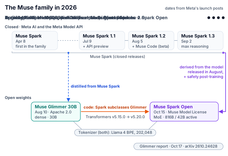
The training arrow points from the closed Muse Spark to Glimmer: Muse Spark is the teacher, Glimmer the student. The code arrow points from Glimmer to Spark Open. Glimmer reached Hugging Face Transformers first (v5.15.0, August 10), and Spark Open’s implementation, which landed in v5.20.0 on October 15, is written against it as a “modular” file. A modular file declares only what differs from existing classes, and a converter expands it into the full modeling file that runs. In modular_muse_spark.py, 18 of the 30 classes subclass a Muse Glimmer class (our count), for example class MuseSparkTextDecoderLayer(MuseGlimmerTextDecoderLayer). That is why this post can teach the shared skeleton once, mostly through Glimmer, whose report explains its choices, and then walk through what Spark changes.

Implementation notes: the code lineage

• modular_muse_spark.py imports 17 Muse Glimmer classes and two helper functions (apply_rotary_pos_emb, eager_attention_forward). From other model families it takes DeepseekV3Experts (parent of MuseSparkExperts), MiniMaxM2TopKRouter (parent of MuseSparkTopkRouter), CLIPMLP (the audio encoder’s multilayer perceptron, MLP), and two Voxtral-Realtime classes, a causal 1-D convolution and its padding cache.
• The vision tower is literally class MuseSparkVisionModel(MuseGlimmerVisionModel): pass. The one vision change sits in MuseSparkVisionPatchEmbedder, which hands the position-table lookup the patch grid as (t, w, h) instead of (t, h, w); the result changes only for non-square images (§6.1). The other 12 classes have no Glimmer parent: the router and experts above, MuseSparkMoE, MuseSparkResidualGate, and the audio config and tower.
• Glimmer is assembled the same way from older models: config, decoder layer, centered RMSNorm, MLP and rotary embedding from Gemma 2; gated attention from AFMoE (AfmoeAttention); the optional-weight RMSNorm from Gemma 4; the vision encoder layers and the multimodal wrapper from Kimi-K2.5; the patch embedder from PaddleOCR-VL.
• models/muse_glimmer first appears at tag v5.15.0 (release, 2026-08-10) and models/muse_spark at v5.20.0 (release, 2026-10-15, via PR #49644).

1.2 Spark Open and Glimmer side by side

How different are the two models on paper? They share the vocabulary, the attention window, the rotary base and the logit cap, and differ in depth, width, head layout, feed-forward block and residual path.

Four terms recur in the tables, and each gets a full section later. A local layer is a sliding-window attention layer: each token attends to itself and the previous 2,047 tokens, and queries and keys carry RoPE. A global layer attends to every earlier token and uses no positional encoding (NoPE); §2.2 explains why the global layers sit at indices 1, 5, …, 61 in Spark (counting from 0) but 3, 7, …, 51 in Glimmer, and §3.4 why they skip RoPE. The latent MoE is Spark’s mixture-of-experts layer: it squeezes each token from 8,192 to 4,096 numbers before the experts and widens it back afterward (§4). The residual gate replaces the plain residual add with a learned per-channel mix of the stream and the sublayer output (§5.2).

The first table lists every structural setting of the two models with the config key it comes from. “Same” means both config.json files hold the same value, byte counts assume BF16, 2 bytes per value, and rows marked “derived” are our arithmetic.

	Muse Spark Open	Muse Glimmer 30B	Config key
Decoder blocks	62	52	num_hidden_layers
Hidden width	8,192	6,656	hidden_size
Query heads / KV heads	128 / 16 (8 per KV head)	32 / 2 (16 per KV head)	num_attention_heads, num_key_value_heads
Head dimension	64	128	head_dim
Attention width, heads × head dim (derived)	8,192	4,096	–
KV cache per token per layer, BF16 (derived)	4 KiB	1 KiB	–
Local : global layers	46 : 16 (2.875 : 1)	39 : 13 (3 : 1)	layer_types
Global layers, 0-based (no RoPE)	1, 5, 9, …, 61	3, 7, 11, …, 51	layer_types, layer_rope_theta
Sliding window	2,048 tokens	same	sliding_window
RoPE	θ = 500,000, local layers only	same	rope_parameters, layer_rope_theta
Max positions	1,048,576	131,072	max_position_embeddings
Vocabulary	202,048	same	vocab_size
Feed-forward block	latent MoE in every block: 256 routed SwiGLU (Swish-gated linear unit) experts, top-8, each running at width 4,096 with intermediate width 4,096	dense SwiGLU, 6,656 → 19,968 → 6,656	num_local_experts, num_experts_per_tok, moe_hidden_size, moe_intermediate_size / intermediate_size
Shared experts	0	–	num_shared_experts
QK-norm	weightless RMSNorm on each query and key head, then Q × 5.4730064863875	same, then Q × 3.87	qk_scale_factor
Attention output	weightless per-head output norm (o_norm), then a sigmoid output gate	sigmoid output gate	(code)
Norms around each sublayer	before both sublayers: RMSNorm with gain $1 + w$ (“centered”); after attention: weightless RMSNorm; after the MoE: an “input-scaled” RMSNorm that scales first and normalizes last	sandwich norms: centered RMSNorm before and after each sublayer	rms_norm_eps 1e-5, post_norm_eps 1e-8
Residual connection	learned residual gate, temperature 0.3	plain add	residual_gate_temperature
Logit multiplier (output head; Spark’s router reuses it)	0.17678 = 1/√32	0.19612 = 1/√26	output_multiplier
Final logit softcap	20	same	final_logit_softcapping
Tied embeddings	no	no	tie_word_embeddings
Inputs	text, image, video, audio	text, image (video as frames, “not explicitly optimized for video”)	model cards; report
Perception Encoder	vision transformer (ViT), 50 layers, width 1,536, patch 14, “1.8B” parameters	same architecture; kept frozen during Glimmer’s training	vision_config
Audio encoder	4-stage convolutional stack, 117,840,384 parameters (derived), one token per 1,920 samples (80 ms at 24 kHz)	none	audio_config

The second table covers size and release; GGUF is llama.cpp’s file format. The decoder-block counts are ours, computed from the shapes above.

	Muse Spark Open	Muse Glimmer 30B
Official size	“816B total / 42B active”	“~29.6B” total; “30B” in the name
Decoder blocks (derived)	816,680,173,568 total; 42,780,753,920 active (5.24%)	25,165,111,296, all active (report: “~25.16B”)
Full checkpoint (Hugging Face count)	822,036,529,664	29,776,626,688
Official checkpoints	BF16, 1.644 TB (derived; docs: “about 1.65 TB”); NVFP4, 533.0 GB (derived)	BF16, 59.55 GB (derived; docs: “Around 60 GB”); GGUF Q4_K_M ~17 GB and Q4_K_XL ~20 GB; ExecuTorch exports; a DFlash speculative-decoding drafter (§8)
Access and license	download after accepting the license; Muse Model License	open download; Apache 2.0
Release date	October 15, 2026	August 10, 2026
In Transformers since	v5.20.0	v5.15.0

Where the numbers come from

• Configs. Glimmer’s values come from its official config.json. Spark Open’s values come from the defaults of MuseSparkTextConfig in Transformers v5.20.0 and from the config.json in mlx-community’s public MLX conversion, which redistributes the model under the Muse Model License and adds only quantization keys; the two agree on every structural value in the table except num_shared_experts, a key the code neither defines nor reads (§4.5). Both cards restate the main rows; Spark’s describes “output gate and output norm on the attention block; QK-norm enabled.”
• Global layers and window. Both config docstrings put a NoPE layer at “every 4th layer counted backward from the last,” and in both released configs the full-attention layers are exactly the NoPE layers. A layer $i$ of $L$ is global when $L - 1 - i$ is a multiple of 4; $61 \bmod 4 = 1$ puts Spark’s first global layer at index 1, and $51 \bmod 4 = 3$ puts Glimmer’s at index 3 (§2.2). In the Transformers masks, a local layer sees the current token plus the previous 2,047.
• Derived shapes. KV cache per token per layer = 2 (K and V) × KV heads × head dimension × 2 bytes: 2 × 16 × 64 × 2 = 4,096 B (Spark) and 2 × 2 × 128 × 2 = 1,024 B (Glimmer). The logit multiplier follows the rule both config docstrings give “for the released checkpoint,” 1/√(hidden_size/256).
• Parameter counts. §2.3 derives the decoder-block counts (62 × 13,172,260,864 total, 62 × 690,012,160 active) and reconciles both Hub totals to the parameter. In short: the official “816B / 42B” match the 62 decoder blocks alone, truncated (816.68B and 42.78B would round to 817B and 43B). That convention is our reading; the Glimmer report uses it for its “~25.16B” (“excluding embedding and output layers”). The Hub totals add the untied embedding and head, the final norm, the encoders and, for Spark, the routers’ 15,872-entry FP32 (32-bit floating-point) bias buffer. The Glimmer card’s “~29.6B” equals the sum of the report’s rounded parts (25.16 + 1.34 + 1.34 + 1.8 = 29.64), and “30B” is the checkpoint’s 29.78B rounded.
• Bytes. Spark BF16 is the sum of the 65 shard sizes on the Hub, 1,644,333,393,864 B; NVFP4 follows from the Hub’s per-dtype counts and the split between quantized and BF16 tensors (§4.5, §7.4); Glimmer’s weight index gives 59,553,253,376 B. Doc figures: Spark Open docs, Glimmer “get the model”.

1.3 One skeleton, two answers

What do the two models share, and what does Spark change? Strip away the sizes and almost all of the machine is common to both:

• The attention block. Grouped-query attention, a weightless QK-norm with a fixed multiplier on the queries, and a sigmoid output gate computed from the normed layer input (§3). The two multipliers give both head sizes the same attention temperature, the fixed scale on every attention logit: 3.87 × √128 = 5.473 × √64 = 43.78 (derived; §3.2).
• The layer schedule. Three local layers (window 2,048, RoPE θ = 500,000) per global layer without positions, counted back from the last layer (§2.2, §3.4).
• The norm skeleton. A weightless norm on the token embeddings, a centered RMSNorm before each sublayer, a norm on each sublayer’s output, and an output head scaled by 1/√(d/256) and soft-capped at 20 (§5).
• Vocabulary and vision. The 202,048-token vocabulary, untied embeddings, and the same Perception Encoder architecture, pixel shuffle and adapter (§6.1–6.2).

Spark changes four things:

1. An output norm in attention. A weightless per-head RMSNorm (o_norm) normalizes the attention output before the gate (§3.3).
2. Residual gates and reworked post-norms. Each residual add becomes a learned gate $\alpha \odot x + \beta \odot f$ of the stream $x$ and the branch output $f$, with $\alpha$ and $\beta$ tied so that $\alpha^2 + \beta^2 = 1$ per channel (up to a small clamp). The post-attention norm loses its weight, and the post-FFN norm scales before it normalizes (§5.2–5.3).
3. A latent MoE in place of the dense FFN. A router reads the full 8,192-wide stream and picks 8 of 256 experts; the block pools the token down to 4,096, runs the experts there, and unpools back to 8,192 (§4).
4. An audio encoder. A convolutional stack of 117.84M parameters (derived) turns raw 24 kHz audio into one token per 80 ms (§6.3).

Everything else is the shared design resized: 62 blocks instead of 52, width 8,192 instead of 6,656, 128 query heads of width 64 instead of 32 of width 128, and 1,048,576 positions instead of 131,072.

Why would the same skeleton end up dense in one model and with 256 experts per layer in the other? For the small model, Glimmer’s report gives the answer the introduction quoted. It compared a ladder of dense models against two MoE ladders (1:8 and 1:16 active experts) “keeping the total memory footprint at inference fixed,” and the MoE ladders lost even though the same GPU-hours trained them on several times as many tokens per parameter; §4.6 walks through the experiment and its figure. Our interpretation, which §4.6 develops: when memory caps the total parameter count, every idle expert takes memory but adds nothing to the work a token gets, so at 32 GB a dense model gets more out of each byte.

Spark Open is served without that ceiling. Meta’s docs serve the BF16 checkpoint on eight GPUs and the NVFP4 one “on a single 4-GPU NVIDIA Blackwell node.” On such nodes, in our reading, the cost that grows with every request is compute per token, not stored bytes. Spark spends its parameters accordingly: the routed experts of all 62 layers hold 798.86B of the 816.68B decoder-block parameters (97.8%), and a token activates 42.78B, or 5.24% (both derived). Against Glimmer, Spark stores 32.5× as many decoder-block parameters but activates only 1.70× as many per token (derived). Pooling to the 4,096-wide latent then halves each expert’s parameters and floating-point operations (FLOPs) compared with experts at the full 8,192 width (§4.3).

So the two models are one skeleton with two answers to one question: how to spend feed-forward parameters under the constraint that binds. Under a memory ceiling, spend all of them on every token; with memory to spare, store many experts and touch a few. That framing is our interpretation, and the Glimmer report supports its first half.

---

2. A Tour of the Layers

What happens to one token on its way through Muse Spark Open? It becomes a vector of 8,192 numbers, climbs 62 decoder blocks that all have the same shape, and leaves as 202,048 vocabulary scores. Muse Glimmer 30B makes the same trip with 6,656 numbers and 52 blocks. Inside one model the blocks differ in only one way: whether their attention is local or global. Between the two models the differences sit in a few places inside the block. This section walks the path once, lays out the layer schedule, and counts where the parameters live; §3–§5 then open each part.

2.1 The path of a token

Here is the trip through Spark, with Glimmer’s values in parentheses. The shapes come from the two configs (Glimmer’s and Spark’s, from mlx-community’s MLX conversion, §1.2). The order of operations comes from the Transformers implementation in v5.20.0 (Spark, Glimmer). “Hidden state” means the vector that carries the token between blocks, and RMS is its root mean square.

1. Embedding. The token ID picks one row of a 202,048 × 8,192 table (202,048 × 6,656).
2. Embedding norm. A weightless RMSNorm divides the row by its RMS. There is no learned gain and no $\sqrt{d}$ multiplier like the one Gemma 2’s code applies, so every token enters the stack with RMS 1.
3. Other modalities. Images and video (and, in Spark, audio) go through their own encoders, come out at the same width, pass a weightless RMSNorm just as the token rows do, and overwrite placeholder tokens in the sequence (§6). From here on the stack sees one sequence of vectors.
4. Pre-norm, then attention. A centered RMSNorm (normalize, then multiply each channel by a learned gain $1 + w$) feeds gated grouped-query attention: 128 query heads and 16 key/value heads of width 64 (32 and 2 of width 128). Queries and keys pass a weightless QK-norm, and the queries are then multiplied by a fixed constant (§3.2); local layers rotate queries and keys with RoPE, global layers do not. A sigmoid output gate, computed from the same normed input, scales the result channel by channel before the output projection. Spark adds one step that Glimmer lacks: it normalizes each head’s output (o_norm) before the gate (§3.3).
5. Post-norm, then residual. Spark normalizes the attention output with a weightless RMSNorm, so it leaves at RMS 1 (Glimmer: a centered RMSNorm with a learned gain). Spark’s residual gate then mixes the old hidden state $x$ and the branch output $f$ as $\alpha \odot x + \beta \odot f$, with per-channel coefficients, computed from one learned vector, that satisfy $\alpha^2 + \beta^2 = 1$ up to a small clamp (Glimmer: a plain $x + f$; §5.2).
6. Pre-norm, then feed-forward. Another centered RMSNorm, then Spark’s latent MoE. A router reads the full 8,192-wide vector and picks 8 of 256 experts; a linear projection pools the vector down to 4,096 numbers, the 8 experts run entirely at that width, and a second projection unpools their weighted sum back to 8,192 (§4). (Glimmer: one dense SwiGLU, 6,656 → 19,968 → 6,656.)
7. Post-norm, then residual. Spark’s post-FFN norm is “input-scaled”: it multiplies by its gain first and normalizes last, so this branch also leaves at RMS 1 (Glimmer: a centered RMSNorm). A second residual gate follows (Glimmer: a plain add).
8. Repeat steps 4–7 in all 62 blocks (52).
9. Final norm and head. An RMSNorm with a learned absolute gain, then an untied lm_head from 8,192 numbers to 202,048 scores (from 6,656). It does not reuse the embedding table.
10. Logit scale and cap. The scores are multiplied by output_multiplier $= 1/\sqrt{d/256}$, which is $1/\sqrt{32} \approx 0.1768$ ($1/\sqrt{26} \approx 0.1961$), and soft-capped as $20\tanh(z/20)$, so no final logit leaves the interval $(-20, 20)$ (§5.4).

Every block wraps both sublayers, attention and feed-forward, in a norm before and a norm after: the sandwich norms Glimmer inherits from Gemma 2. Spark keeps the sandwich but changes the post-norms: both now end with a normalization and no weight after it, so both branches always write a unit-RMS vector. In our reading, the residual gate’s norm-preserving arithmetic depends on that (§5.2).

In plain terms, follow one Spark token through layer 1, which is a global layer (§2.2). The pre-norm scales its 8,192 numbers to RMS 1, a length of $\sqrt{8{,}192} \approx 90.5$, before applying its learned gain. The projections turn the result into 8,192 query numbers (128 heads × 64), 1,024 key and 1,024 value numbers (16 heads × 64), and 8,192 gate values. The 2,048 key and value numbers, 4 KiB in BF16, are what the token leaves in this layer’s cache, and because layer 1 is global they stay there for the whole sequence. In a channel where the post-attention residual gate sits at $\beta = 0.5$ (gate parameter 0), the new hidden state in that channel is $0.866\,x + 0.5\,f$, since $\alpha = \sqrt{1 - 0.5^2}$. Then the router scores 256 experts and keeps 8. The pooled 4,096-number vector enters each chosen expert, is widened to 2 × 4,096 inside (the gate and up halves of SwiGLU), and comes back as 4,096 numbers. The token touched 8 × 50,331,648 ≈ 402.7M of the block’s 12.88B expert weights, 3.1% (derived), about as many as Glimmer’s whole dense FFN (§4.1).

Three things common in recent large MoE models are missing from this list. There is no MTP layer: the counts in §2.3 match both checkpoints with nothing left over, and speculative decoding uses separate drafter models built on DFlash or a close relative instead (§8). Spark has no dense layers: all 62 blocks are sparse (§4.5). And Spark has no shared expert: all 256 experts are routed (§4.5). Neither model has attention biases, an attention-logit soft-cap or learned attention sinks, the extra per-head logits some models add so that a head can put its attention weight on no token at all (§3.3–3.4).

Implementation notes

• Call chain. MuseSparkForConditionalGeneration.forward calls MuseSparkModel.forward, which zeroes the image, video and audio placeholder IDs (llm_input_ids[multimodal_mask] = 0), embeds the sequence, and writes the encoder outputs over the placeholders with inputs_embeds.masked_scatter(...). MuseSparkTextModel.forward runs the 62 blocks and the final self.norm. Back in the top class come self.lm_head(...), logits * output_multiplier, then a division by final_logit_softcapping (20), torch.tanh and a multiplication by 20.
• Embedding. MuseSparkTextNormedEmbedding is an nn.Embedding whose forward returns self.embed_norm(super().forward(input_ids)). The norm stays a separate module so that the DFlash drafter can embed without it (§5.4). Spark’s audio features pass through this same embed_norm; vision features pass through perception_emb_norm, a separate module with the same math.
• The block. The body of MuseSparkTextDecoderLayer.forward, with the attention call’s keyword arguments shortened:

residual = hidden_states
hidden_states = self.input_layernorm(hidden_states)
hidden_states, _ = self.self_attn(hidden_states=hidden_states, ...)
hidden_states = self.post_attention_layernorm(hidden_states)
hidden_states = self.post_attention_residual_gate(residual, hidden_states)
residual = hidden_states
hidden_states = self.pre_feedforward_layernorm(hidden_states)
hidden_states = self.mlp(hidden_states)
hidden_states = self.post_feedforward_layernorm(hidden_states)
hidden_states = self.post_feedforward_residual_gate(residual, hidden_states)

• The classes behind those names. MuseSparkTextCenteredRMSNorm for both pre-norms, MuseSparkRMSNorm(..., with_scale=False) after attention, MuseSparkTextInputScaledRMSNorm after the FFN, two MuseSparkResidualGates, and MuseSparkMoE, built when config.mlp_layer_types[layer_idx] == "sparse". Glimmer’s MuseGlimmerTextDecoderLayer runs the same sequence with residual + hidden_states in place of the gates and centered norms in all four places.
• Written as a diff. Spark’s block and attention subclass Glimmer’s, which in turn subclass Gemma2DecoderLayer and AfmoeAttention; the router and experts start from MiniMaxM2TopKRouter and DeepseekV3Experts. §1.1’s notes list every parent class in modular_muse_spark.py.
• Precision. _keep_in_fp32_modules_strict lists post_attention_residual_gate, post_feedforward_residual_gate, mlp.gate.weight and e_score_correction_bias, so routing and the gate coefficients run in FP32, while in a BF16 run the hidden state itself stays BF16 (§5.2).
• llama.cpp. muse-spark.cpp builds the same graph, and the converter folds the static pieces into the weights: the $+1$ of each $1 + w$ gain, the query scale (into a synthesized Q-norm weight), the router’s logit multiplier, and the gate coefficients $\alpha$ and $\beta$.

2.2 The layer schedule: three local, one global

Which layers are local and which are global? Both configs carry an explicit list, layer_types, and both code defaults generate it with the same rule: layer $i$ of $L$ is global when

\[(L - 1 - i) \bmod 4 = 0 ,\]

and local otherwise. The config docstring describes the same layers in words: NoPE on “every 4th layer counted backward from the last”. Because the count starts at the top, the index of the first global layer depends on $L$. The table shows the result for both models.

	Decoder blocks	Global layers (0-based)	Local : global
Muse Glimmer 30B	52 = 4 × 13	3, 7, 11, …, 51	39:13 = 3:1
Muse Spark Open	62 = 4 × 15 + 2	1, 5, 9, …, 61	46:16 = 2.875:1

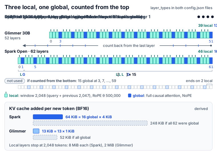
Glimmer’s 52 is a multiple of 4, so counting back from layer 51 lands on 3, 7, …, 51, and the pattern [local, local, local, global] repeats cleanly from layer 0. The Glimmer report’s architecture table puts it the same way: “[Local, Local, Local, Global] repeating”. Spark’s 62 leaves a remainder of 2. Counting back from layer 61 lands on 57, 53, …, 5, 1: layer 0 is local, layer 1 is already global, and then [L, L, L, G] repeats fifteen times. That gives 16 global and 46 local layers. A forward rule, $(i + 1) \bmod 4 = 0$, would have given Spark 15 global layers at 3, …, 59 and ended the stack on two local layers (derived).

Both stacks end on a global layer, so the last layer before the output head always reads the whole context. That is our reading of why the count starts at the top.

The two kinds of layer differ in what they read and in how they handle position. A local layer attends to a sliding window of 2,048 positions, the token itself plus the previous 2,047, and rotates queries and keys with RoPE (θ = 500,000, no scaling). A global layer attends to every earlier token and has no positional encoding. §3.4 covers the window semantics and why the global layers skip RoPE, the choice that, in our reading, lets Spark serve 1M positions without RoPE scaling (§7.1).

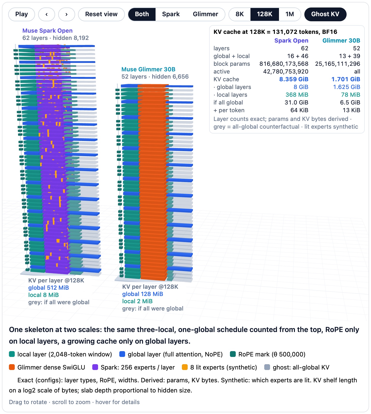
The schedule also sets the memory bill (derived). A local layer’s cache stops growing at its window, so only the global layers grow: each new token adds 16 × 4 KiB = 64 KiB to Spark’s cache (248 KiB if all 62 layers were global) and 13 × 1 KiB = 13 KiB to Glimmer’s (52 KiB). §7.2 works through the full table, up to 64.4 GiB for one 1M-token Spark sequence.

The rhythm has relatives, and all three below count it from the bottom. Meta’s Llama 4 uses “interleaved attention layers without positional embeddings”, and its Transformers config places them with the forward rule, NoPE where $(i + 1) \bmod 4 = 0$. Cohere’s RNoPE-SWA (arXiv 2501.18795) interleaves sliding-window RoPE layers with full-attention NoPE layers; it found that “a 1:3 ratio strikes an optimal balance” and puts the full-attention layer “at the end of each interleaving group”. §3.4 compares both designs with Muse. GLM-5.3-Flash uses the same three-then-one rhythm, three Kimi Delta Attention (KDA) layers per DeepSeek Sparse Attention (DSA) layer, and, unlike Muse, counts from the bottom, so its stack ends on a trailing KDA layer (GLM-5.3 post, §8.1).

The animation below lines up the two schedules at their last layer. Read it from the right: the global columns coincide in both stacks, and only the two leftover layers at the bottom of Spark’s stack shift its first global layer to index 1. The dashed strip shows the unused forward rule ending Spark on two local layers; the last two beats add RoPE ticks on the local layers and the cache each new token adds.

Read the strips from the right: both models make every fourth layer, counted back from the last, a global NoPE layer (Glimmer 39:13 with globals 3, 7, …, 51; Spark 46:16 with globals 1, 5, …, 61), so the global columns line up and only Spark’s two leftover bottom layers move its first global layer to index 1; the dashed forward-rule strip is a counterfactual the model does not use, and the per-token cache figures (64 vs 248 KiB, 13 vs 52 KiB) are derived from the configs. Open the full-size SVG.

Implementation notes

• Config rule. MuseSparkTextConfig.__post_init__ (Glimmer’s config class uses the identical rule) builds layer_types with "full_attention" if (self.num_hidden_layers - 1 - i) % 4 == 0 else "sliding_attention", under the comment “the reference config’s sliding_window_pattern [w, w, w, 0]”. layer_rope_theta uses the same test to put 0 (NoPE) on those layers and 500,000 everywhere else. Both released config.json files spell out the two lists, and both match the rule.
• Per block. MuseSparkTextModel.forward builds two masks once, create_causal_mask and create_sliding_window_causal_mask, and passes each block causal_mask_mapping[self.config.layer_types[i]] and position_embeddings if self.config.layer_rope_theta[i] else None. Only the truthiness of layer_rope_theta matters: one rotary table, built from the global rope_theta, serves every local layer. §3.4 quotes the mask and sliding-cache code behind “the token itself plus the previous 2,047”.
• llama.cpp. Spark’s loader requires the explicit per-layer pattern (ml.get_arr(LLM_KV_ATTENTION_SLIDING_WINDOW_PATTERN, hparams.is_swa_impl)), RoPE runs where use_rope = hparams.is_swa(il), and the converter asserts sliding == [bool(t) for t in hparams["layer_rope_theta"]]. Glimmer’s loader can fall back to a period-4 pattern (load_swa_pattern(ml, 4), global where il % 4 == 3). That fallback is right for 52 layers only because 52 is a multiple of 4; for Spark it would put the globals at 3, …, 59 (derived).

In the 3D model below, the two stacks stand side by side with layer 0 at the bottom: teal slabs are local layers, blue slabs global ones, and RoPE marks run beside the local layers only. Switch the context between 8K, 128K and 1M and watch the KV shelf next to each slab (drawn on a log scale). Local shelves stop at 2,048 tokens (8 MiB per layer in Spark, 2 MiB in Glimmer) while global shelves keep growing; at 1M Glimmer greys out, because its config stops at 131,072 positions. Turn on the ghost shelves to see the all-global counterfactual (248 GiB for Spark at 1M), and step to the last beat to compare the feed-forward parts: one dense block per layer in Glimmer, a 16 × 16 grid of experts with 8 lit in Spark (the lit experts are a synthetic choice).

Switch the context to 1M to see that only Spark's 16 global layers keep growing their KV shelves (Glimmer stops at 128K), press Ghost KV for the all-global counterfactual, or step through the five beats; layer types and RoPE marks are exact from the configs, parameter counts and KV bytes are derived from them, the lit experts are a synthetic choice, and shelf length is on a log2 scale.

2.3 Where the parameters live

Spark keeps almost all of its weights in routed experts, and a token uses about one in 19 of its decoder-block parameters. Glimmer keeps most of its weights in a dense FFN and uses all of them. The tables below are our count from the config shapes, and the count reproduces both public checkpoints to the parameter. The first table covers one decoder block.

Per decoder block (derived)	Spark Open	Glimmer
q_proj	67,108,864	27,262,976
k_proj + v_proj	16,777,216	3,407,872
o_proj	67,108,864	27,262,976
gate_proj (output gate)	67,108,864	27,262,976
Attention	218,103,808	85,196,800
Routed experts (256 × 50,331,648) / dense SwiGLU	12,884,901,888	398,721,024
Router (256 × 8,192)	2,097,152	—
Pool and unpool projections (2 × 8,192 × 4,096)	67,108,864	—
Pre- and post-expert norm gains (2 × 4,096)	8,192	—
Feed-forward	12,954,116,096	398,721,024
Block norm gains	24,576 (3 × 8,192)	26,624 (4 × 6,656)
Residual gates	16,384 (2 × 8,192)	—
Block total	13,172,260,864	483,944,448
Active per token	690,012,160 (8 of 256 experts)	483,944,448 (all)

The second table scales the block up to the whole model and adds the parts outside the stack.

Whole model (derived)	Spark Open	Glimmer
Decoder blocks	62 × 13,172,260,864 = 816,680,173,568	52 × 483,944,448 = 25,165,111,296
Token embedding (202,048 × $d$)	1,655,177,216	1,344,831,488
lm_head (untied, same shape)	1,655,177,216	1,344,831,488
Final norm	8,192	6,656
Perception Encoder (vision tower)	1,852,639,744	1,852,639,744
Vision adapter + projection	75,497,472	69,206,016
Audio encoder	117,840,384	—
Parameters	822,036,513,792	29,776,626,688
Router bias buffers (62 × 256, stored in FP32)	15,872	—
Stored values	822,036,529,664	29,776,626,688
Hugging Face API count	822,036,529,664	29,776,626,688
Active per token, decoder blocks	42,780,753,920	25,165,111,296

What do the official sizes count? Spark’s model card says “816B total / 42B active”. Our decoder-block counts, 816.68B and 42.78B, would round to 817B and 43B, and adding the embedding and head would give 819.99B. The official figures therefore match the decoder blocks alone, truncated to whole billions (our inference). The Hub’s 822,036,529,664 for the Spark repo counts every stored value, including the 15,872 entries of e_score_correction_bias, the router’s selection bias. That tensor is a buffer, not a parameter: it receives no gradient (§4.2), so our 816,680,173,568 leaves it out.

Glimmer’s figures include the embeddings and the encoder. The report’s architecture table lists “~29.6B” in total: ~25.16B in transformer blocks, ~1.34B each for the untied embedding and output projection, and ~1.8B for the Perception Encoder, and the model card gives “29.6B (including vision encoder)”. Our block count, 25,165,111,296, matches the ~25.16B. The listed parts sum to 29.64B; the checkpoint’s 29.78B also holds the encoder’s exact 1.853B and the 69.2M vision adapter and projection (derived). “30B” rounds the checkpoint up.

The shares show the shape of each model: routed experts hold 97.8% of Spark’s block parameters; a token uses 5.24% of all block parameters (3.1% of the expert weights); and Glimmer’s dense FFN holds 82.4% of its own (all derived).

On the active side, attention is a much larger slice of Spark: 13.52B of 42.78B active block parameters (31.6%), against 4.43B of 25.17B in Glimmer (17.6%, derived). A matrix-vector product costs two operations per weight, so these are also attention’s shares of the per-token matmul compute at short context; the score computation over cached keys comes on top and grows with context (§7.3). Two shape choices explain the gap. Spark’s attention is square: its query, gate and output projections all map 8,192 numbers to 8,192, while Glimmer’s run between 6,656 and a narrower 4,096 (§3.1). And Spark’s FFN is sparse, so per token it is small: its 8 active experts hold 402.7M weights per block, about the size of Glimmer’s whole dense FFN (§4.1), plus 67.1M for the pool and unpool projections. Per token, Spark’s blocks do 1.70× the matmul work of Glimmer’s (derived). Within attention, the output gate is as large as q_proj and takes almost a third of the weights in both models (§3.3).

Derivation

• Attention per block. With hidden size $d$, $n_q$ query heads, $n_{kv}$ KV heads and head width $h$, the four projections hold $d\,n_q h$ (q) $+\ 2\,d\,n_{kv} h$ (k, v) $+\ n_q h\,d$ (o) $+\ d\,n_q h$ (gate). Spark: $3 \times 8{,}192 \times 8{,}192 + 2 \times 8{,}192 \times 1{,}024 = 218{,}103{,}808$. Glimmer: $3 \times 6{,}656 \times 4{,}096 + 2 \times 6{,}656 \times 256 = 85{,}196{,}800$. There are no biases (attention_bias: false), and QK-norm and o_norm have no weights. The output gate is 30.8% of Spark’s attention weights and 32.0% of Glimmer’s.
• Spark’s feed-forward. One expert is $3 \times 4{,}096 \times 4{,}096 = 50{,}331{,}648$ (gate_up_proj [8,192, 4,096] plus down_proj [4,096, 4,096]). Add 256 experts, the router ($256 \times 8{,}192$), the pool and unpool projections ($2 \times 8{,}192 \times 4{,}096$) and two 4,096-wide norm gains: 12,954,116,096. Active: 8 experts instead of 256, which gives 471,867,392. The post-expert norm is one 4,096-wide gain shared by all 256 experts of a layer, so it counts once.
• Glimmer’s FFN. $3 \times 6{,}656 \times 19{,}968 = 398{,}721{,}024$.
• Norms and gates. Spark has three weighted block norms (input, pre-FFN and post-FFN; the post-attention norm has no weight) and two residual gates of 8,192 each: 40,960. Glimmer has four weighted norms: 26,624.
• Embedding and head. $202{,}048 \times d$ each: 1,655,177,216 for Spark (the card gives “≈ ~1.66B”) and 1,344,831,488 for Glimmer (the report’s “~1.34B”). The final norm adds $d$.
• Perception Encoder. 50 layers × 36,985,088, plus the patch embedding (1,806,336), the 32 × 32 position table (1,572,864) and two outer LayerNorms (6,144): 1,852,639,744 in both models (§6.1). Adapter and projection: $6{,}144 \times 4{,}096 + 4{,}096 \times 4{,}096 + 4{,}096 \times d$, which is 75,497,472 for Spark and 69,206,016 for Glimmer.
• Audio encoder (Spark). Four convolution stages of 1,060,352, 4,996,096, 19,429,376 and 75,558,912 parameters, plus an output head of 16,795,648: 117,840,384 (§6.3).
• Checkpoint dtypes. The Hub lists {'BF16': 821906490368, 'F32': 130039296} for Spark. The F32 part is exactly $62 \times (256 \times 8{,}192 + 256)$: the router weights plus the bias buffers. The Hub lists all 29,776,626,688 of Glimmer’s values as BF16.
• Active counts leave out the embedding lookup (one row per token) and the lm_head. With the head, Spark’s active count is 44,435,931,136.
• Shares. Attention: $62 \times 218{,}103{,}808 = 13{,}522{,}436{,}096$ of 42,780,753,920 (31.6%); $52 \times 85{,}196{,}800 = 4{,}430{,}233{,}600$ of 25,165,111,296 (17.6%). Routed experts: $62 \times 12{,}884{,}901{,}888 = 798{,}863{,}917{,}056$ of 816,680,173,568 (97.8%). Active fraction: $690{,}012{,}160 / 13{,}172{,}260{,}864 = 5.24\%$. Glimmer FFN: $52 \times 398{,}721{,}024 / 25{,}165{,}111{,}296 = 82.4\%$.

---

3. Attention: Gated GQA with a Fixed Temperature and No Positions on Global Layers

What happens inside one attention sublayer of Muse Spark Open and Muse Glimmer 30B, and how far is it from the textbook version? Not far. Both models start from grouped-query attention and add three things. Queries and keys pass through a per-head RMSNorm with no learned weight, and the query is then multiplied by a fixed constant, so that in both models every attention logit equals 43.784 times a cosine. A sigmoid gate scales every output channel before the output projection. And rotary position embeddings run on local layers only, so global layers see no positions at all. Spark adds a fourth change: a weightless RMSNorm on each head’s output, just before the gate.

The code makes the inheritance literal. In the modular file, MuseSparkTextAttention subclasses MuseGlimmerTextAttention, adds one module in __init__ (self.o_norm) and repeats Glimmer’s forward with one extra call. Everything else here applies to both models; Spark’s numbers come first, Glimmer’s in parentheses.

3.1 GQA shapes and what one token caches

How much does one token cost in one layer’s cache? 4 KiB in Spark and 1 KiB in Glimmer, because both models let many query heads share each key/value head. In multi-head attention (MHA), every query head has its own key head and value head, so each token leaves 2 × heads × head_dim numbers in the KV cache of every layer. Multi-query attention shares one key/value head among all query heads. GQA (Ainslie et al., 2023) sits in between: it “uses an intermediate (more than one, less than number of query heads) number of key-value heads”. The query heads form equal groups, and each group reads one shared key/value head.

Spark has 128 query heads and 16 KV heads of width 64, so each KV head serves 8 query heads. Its attention width, 128 × 64 = 8,192, equals the hidden size. Glimmer has 32 query heads and 2 KV heads of width 128, so each group has 16 heads, and its attention width of 32 × 128 = 4,096 is narrower than its 6,656-wide hidden state. Glimmer’s attention is therefore not square: q_proj and the gate map 6,656 numbers down to 4,096, and o_proj maps 4,096 back up to 6,656. The table lists every weight, from the Spark config (in mlx-community’s public MLX conversion), the Glimmer config and the code; §2.3 places these counts in the whole parameter budget.

Per decoder block	Muse Spark Open	Muse Glimmer 30B
Hidden size	8,192	6,656
Query heads × head_dim	128 × 64 = 8,192	32 × 128 = 4,096
KV heads × head_dim	16 × 64 = 1,024	2 × 128 = 256
Query heads per KV head	8	16
q_proj and gate_proj [out × in]	8,192 × 8,192	4,096 × 6,656
k_proj and v_proj [out × in]	1,024 × 8,192	256 × 6,656
o_proj [out × in]	8,192 × 8,192	6,656 × 4,096
Parameters, all five matrices (derived)	218,103,808	85,196,800
KV cache per token (derived)	2,048 values = 4,096 B in BF16	512 values = 1,024 B in BF16

There are no biases: attention_bias is false, and the gate is built with bias=False.

In plain terms: when a token passes through one Spark layer, the layer writes 16 keys and 16 values of 64 numbers each into the cache, 2,048 numbers or 4 KiB in BF16. Glimmer writes 2 keys and 2 values of 128 numbers, 512 numbers or 1 KiB. With one KV head per query head (MHA), the same token would cost 16,384 numbers in Spark (8× more) and 8,192 in Glimmer (16× more) (derived). Only global layers keep these entries for the whole conversation; a local layer drops a token once it falls out of the 2,048-token window (§3.4). §2.2 multiplies this out per new token, and §7.2 turns it into totals.

Why does Glimmer share so aggressively? Inside its 32 GB envelope, the Glimmer report (section “Design for on-device efficiency”) names the cache as the next problem after the weights: “the memory footprint of long-horizon agentic sessions is heavily dominated by the size of the key-value (KV) cache.” Its answers are the sliding window and “grouped-query attention with only 2 KV heads per layer with head dimension of 128.” At 131,072 tokens Glimmer’s BF16 cache is 1.70 GiB; with 8 KV heads instead of 2 it would be 6.8 GiB (derived). That cache has to fit beside a roughly 4-bit language model that the model card puts at “under 20 GB”.

Spark shares less aggressively: it keeps 8 query heads per KV head, with heads half as wide as Glimmer’s.

Implementation notes

• MuseGlimmerTextAttention.__init__ builds q_proj, k_proj, v_proj and o_proj with bias=config.attention_bias and gate_proj with bias=False, and sets num_key_value_groups = num_attention_heads // num_key_value_heads (8 or 16). The eager reference path expands each KV head to its group with repeat_kv. The flash backend takes the shared heads directly; the SDPA backend (PyTorch’s scaled_dot_product_attention) passes enable_gqa=True when the PyTorch build and mask allow it and falls back to repeat_kv otherwise.
• Checkpoint layout: Glimmer’s public weight index lists exactly self_attn.{q,k,v,o,gate}_proj.weight under each layer, with no norm or bias tensors. For Spark, the community MLX 3-bit index shows a fused self_attn.qkvg_proj plus o_proj (names chosen by the converter), also without norm tensors.

3.2 Scaleless QK-norm and one temperature

How large can an attention logit get? In Muse, never larger than 43.784 in magnitude. In textbook attention, a logit is $q \cdot k / \sqrt{d}$, and nothing in that formula limits the size of $q$ or $k$. During training they can grow, the logits grow with them, and the softmax turns into a near one-hot choice. ViT-22B hit exactly this: “extremely large values in attention logits, which lead to (almost one-hot) attention weights with near-zero entropy” (arXiv 2302.05442). Gemma 2 capped attention logits with a tanh at 50.0 (arXiv 2408.00118); Gemma 3 “replace[d] the soft-capping of Gemma 2 with QK-norm” (arXiv 2503.19786), normalizing queries and keys before the dot product. Muse takes the second route. Glimmer’s config class in the modular file even subclasses Gemma2Config and deletes its attention soft-cap field, attn_logit_softcapping.

The order of operations in MuseSparkTextAttention.forward, which Glimmer shares:

1. Project and split into 128 query heads of 64 numbers (32 × 128) and 16 key and 16 value heads (2 and 2).
2. Normalize each head. Every query head and key head is divided by its own root mean square, $\hat{x} = x / \sqrt{\mathrm{mean}(x^2) + 10^{-5}}$, in FP32. There is no learned weight; one weightless module serves both Q and K. Values are not normalized.
3. Scale the query only by qk_scale_factor: 5.4730064863875 in Spark, 3.87 in Glimmer. The config docstring calls it a “Multiplier applied to Q after the scaleless QK-norm, on top of the standard 1/sqrt(head_dim) attention scaling.”
4. Rotate (local layers only). RoPE (§3.4) is a rotation, so lengths are unchanged.
5. Attend, multiplying $q \cdot k$ by the usual $1/\sqrt{d}$ before the softmax.

After step 2 a vector of $d$ numbers with RMS 1 has length $\sqrt{d}$, so two such vectors have dot product $d \cos\theta$, where $\theta$ is the angle between them. With $s$ the scale factor:

\[\text{logit} \;=\; \frac{(s\,\hat{q}) \cdot \hat{k}}{\sqrt{d}} \;=\; \frac{s\, d \cos\theta}{\sqrt{d}} \;=\; s\sqrt{d}\,\cos\theta .\]

Spark: $5.4730064863875 \times \sqrt{64} = 43.7840518911$. Glimmer: $3.87 \times \sqrt{128} = 43.7840518911$ (derived). The two configs store different numbers that encode the same thing: in both models every attention logit is $43.784 \cos\theta$, so it always lies between −43.784 and +43.784, whatever the size of the hidden state. As a scale on the raw normalized dot product, that is $43.784/d$: 0.684 for Spark, 0.342 for Glimmer (derived). This fixed multiplier is the “temperature” of this section’s headings. Strictly it is an inverse temperature: it multiplies the logits, where a softmax temperature divides them, so a larger value allows sharper attention.

In plain terms: in one Spark head, let the normalized query and key point the same way. Each has length 8, their dot product is 64, and 64 × 5.473 × 1/8 = 43.78. At 60° apart (cos θ = 0.5) the logit is 21.89. In a Glimmer head the aligned case is 128 × 3.87 × 1/√128 = 43.78 again: heads twice as wide, the same ceiling.

The ceiling does not make attention soft. A perfectly aligned key outweighs an orthogonal one by $e^{43.78} \approx 1.0 \times 10^{19}$, and keys at cos θ = 1 and 0.9 still differ by a factor of about 80 in unnormalized weight (derived). It only stops logits from growing without limit. There is a known trade-off: Cohere’s “Rope to Nope and Back Again” (arXiv 2501.18795) found that QK-norm made logits “flatter in terms of distribution” and hurt needle retrieval, so its authors removed it. Our reading is that Muse keeps QK-norm but fixes a large logit scale (a low softmax temperature), with a ceiling of 43.784 close to Gemma 2’s cap of 50, so sharp attention stays available.

Is the shared 43.784 an accident? Public training code suggests not. TorchTitan’s Muse Spark flavors file defines _SCALE_QUERY_NUMERATOR = 43.7840518911, commented “The query is scaled by this tuned constant divided by sqrt(head_dim) after q-norm”. The 816B flavor sets query_scale=_SCALE_QUERY_NUMERATOR / math.sqrt(64), and the file’s small debugmodel flavor, with head_dim=32, divides the same numerator by math.sqrt(32). Glimmer’s config stores only 3.87; that it is the same constant over √128 is our arithmetic: $3.87 \times \sqrt{2} = 5.4730064863839$, within $3.6 \times 10^{-12}$ of Spark’s value.

What rule could produce it? llama.cpp’s converter calls the multiplier “the MetaP scale” (a contributor’s comment), and Meta’s Llama 4 blog introduced MetaP as a way to set “per-layer learning rates and initialization scales” whose values “transfer well across different values of batch size, model width, depth, and training tokens”. Our reading: holding $s\sqrt{d}$ fixed while head_dim changes looks like such a transfer rule, and the resulting $43.784/d$ is the “1/d attention instead of 1/√d” of maximal update parametrization (µP, arXiv 2203.03466), with a tuned constant in front. µP sets initialization scales, learning rates and multipliers as functions of model width so that hyperparameters tuned on a small model carry over to a large one, and this attention scaling is one of its rules. §5.4 reads the output head the same way.

One older design makes the comparison exact. QKNorm (arXiv 2010.04245) applies “ℓ2 normalization along the head dimension” and scales “by a learnable parameter instead of dividing by the square root of the embedding dimension”. An RMS-normalized vector is √d times an ℓ2-normalized one, so Muse is QKNorm with that parameter frozen at 43.784 (derived).

Implementation notes

• Code: self.qk_norm = MuseSparkRMSNorm(eps=config.rms_norm_eps, with_scale=False), then query_states = self.qk_norm(query_states) * self.qk_scale_factor and key_states = self.qk_norm(key_states). The norm computes hidden_states * torch.pow(mean_squared, -0.5) in FP32 and casts back (§5.3 covers every RMSNorm variant).
• The softmax scale stays self.scaling = self.head_dim**-0.5 (0.125 or 0.0884); the eager kernel computes torch.matmul(query, key_states.transpose(2, 3)) * scaling and the softmax in FP32. Glimmer’s modular file deletes Gemma 2’s query_pre_attn_scalar and the learned norms of its AFMoE parent (del self.q_norm, del self.k_norm).
• The cache update comes after the norm and RoPE, so cached keys have RMS 1 per head.
• The eps lowers the ceiling slightly when the pre-norm vectors are tiny. If query and key both have pre-norm mean square $m$, the bound becomes $43.784\, m/(m + 10^{-5})$: 43.7836 at $m = 1$, 39.80 at $m = 10^{-4}$ (derived). For random directions, typical logits spread by about $s$: 5.47 in Spark, 3.87 in Glimmer (derived approximation). Same ceiling, different typical spread.
• The Transformers Llama 4 code normalizes queries and keys only on RoPE layers (if self.config.use_qk_norm and self.use_rope); Muse does it on every layer.
• llama.cpp’s converters fold the multiplier into synthesized norm weights: a Q-norm weight filled with qk_scale_factor and a K-norm weight of ones, “so the graph keeps the plain 1 / sqrt(head_dim)”.

3.3 The output gate (and Spark’s output norm)

What does the output gate buy, and why does Spark put a norm in front of it? The closest public study (Qiu et al., below) finds that such a gate improves perplexity and training stability and mitigates attention sinks; our reading is that Spark’s extra o_norm leaves the gate alone to decide how loudly each head speaks.

After the softmax-weighted sum, every Muse attention layer multiplies the concatenated head outputs by a sigmoid gate computed from the layer’s input, then applies the output projection (Spark adds one step, described at the end of this subsection):

\[y \;=\; W_O\big(\,\mathrm{attn}(x) \odot \sigma(W_G\, x)\,\big).\]

Three details matter. The gate reads the same input as $q$, $k$ and $v$: the pre-normed hidden state $x$ from the block’s input_layernorm (§2.1), not the attention output. It is element-wise: gate_proj has one output per channel of the concatenated heads, 8,192 (4,096), so every dimension of every head has its own gate, not one scalar per head. And it sits between the attention and o_proj.

In plain terms: Spark’s channel 200 is dimension 8 of head 3 (3 × 64 + 8, counting from 0). Say that head outputs 0.8 there for two consecutive tokens. For the first token the gate logit is −2, σ(−2) = 0.119, and 0.095 goes on to o_proj. For the second the logit is +2, σ(2) = 0.881, and 0.70 goes on. Same head output, different gate: the gate decides, per token and per channel, how much reaches o_proj and, from there, the residual stream.

The gate is not cheap: gate_proj is exactly as large as q_proj, as the table shows.

Output gate (derived from the shapes)	Spark	Glimmer
Parameters per decoder block	67,108,864	27,262,976
Share of attention parameters	30.8%	32.0%
All decoder blocks	4.16B (9.7% of 42.78B active)	1.42B (5.6% of 25.17B)
Matmul FLOPs per token per block (2 per weight)	134.2M	54.5M

Now the evidence behind the opening answer. The Glimmer report states that “Gated attention is applied throughout”, and the Spark model card lists “Gated Attention: Yes (output gate and output norm on the attention block; QK-norm enabled)”. The closest public study is Qiu et al., “Gated Attention for Large Language Models” (2025), which ran “a comprehensive comparison over 30 variants” of 15B MoE and 1.7B dense models trained on a 3.5-trillion-token dataset. Its central finding: “applying a head-specific sigmoid gate after the Scaled Dot-Product Attention (SDPA)—consistently improves performance. This modification also enhances training stability, tolerates larger learning rates, and improves scaling properties.” Their gate is $Y’ = Y \odot \sigma(XW_\theta)$, with a footnote that matches Muse’s choice of input (“We adopt the hidden states after pre-normalization as X”), and their best variant by perplexity, “SDPA Elementwise G1”, has Muse’s shape: element-wise, head-specific, sigmoid.

The paper gives two explanations. One is non-linearity: without a gate, a head’s contribution is $\sum_j S_{ij}\, x_j W_V W_O$, where $S_{ij}$ is query $i$’s softmax weight on token $j$ and $x_j$ is token $j$’s normed input, so $W_V W_O$ acts as one low-rank linear map (rank at most head_dim), further limited when GQA shares $W_V$ across a group; a non-linearity between them adds expressiveness. The other is sparsity: the learned gates are mostly near zero (mean score 0.116), so a head can output almost nothing when it has nothing to add. The paper ties this to the attention sink. Softmax weights must sum to 1, so a head with nothing useful to read still has to put its weight somewhere, and StreamingLLM observed models placing strong attention on initial tokens “as a ‘sink’ even if they are not semantically important”. Qiu et al. find that “this sparse gating mechanism mitigates ‘attention sink’ and enhances long-context extrapolation performance”. In their 15A2B MoE (15B total, 2.54B active) trained on 400B tokens, the gate cut average perplexity from 6.026 to 5.761, the share of attention on the first token from 0.467 to 0.048, and the maximum hidden-state activation (averaged over layers) from 1,053 to 94. These are Qiu et al.’s models, not Muse.

The sink point weighs more in Muse than usual (our reading). Muse has no learned sink logits, unlike DeepSeek-V4 (DeepSeek-V4 post, §3.4). And in a local layer, the sequence’s first token drops out of the window once the query is 2,048 positions past it, so a fixed sink token is not always visible. In Spark, whose o_norm (below) fixes every head’s output at RMS 1, the gate is the only way for a head to say nothing. A Glimmer head could also learn to read near-zero values, but there too the gate is the only built-in off switch.

Spark’s output norm. Spark inserts o_norm between the attention and the gate: a weightless RMSNorm applied to each head’s 64-number output separately. The order becomes attention → o_norm per head → × σ(gate) → o_proj, so every head’s output has RMS 1 (length 8) before the gate scales it.

Why would that help? Our reading: a head’s output is a weighted average of value vectors, and its length carries an accidental signal. Focused attention keeps a value’s length, while diffuse attention over dissimilar values shrinks it. With two orthogonal unit values, (1, 0) and (0, 1), the focused output has length 1 and the even average (0.5, 0.5) has length 0.71. o_norm discards the length and keeps the direction, so the gate alone decides how loudly a head speaks. Qiu et al. tested a per-head RMSNorm alone at the same position (the “SDPA GroupNorm” row of their Table 3): average perplexity 5.847, against 6.026 for their baseline and 5.761 for the gate. RetNet (arXiv 2307.08621) uses the same order Spark does, a per-head norm and then a gate, with GroupNorm and swish where Spark has a weightless RMSNorm and a sigmoid.

Implementation notes

• Code: self.gate_proj = nn.Linear(config.hidden_size, config.num_attention_heads * self.head_dim, bias=False). In forward: attn_output = self.o_norm(attn_output).reshape(*input_shape, -1).contiguous(), then attn_output = attn_output * torch.sigmoid(self.gate_proj(hidden_states)), then self.o_proj(attn_output). Glimmer’s line has no self.o_norm.
• Why per head: the attention backends return [batch, seq, heads, head_dim], and o_norm runs before the reshape, over each head’s 64 numbers. llama.cpp makes it explicit (“Weightless norm on the attention output, applied per head”): a reshape to [n_embd_head, n_head, n_tokens], then ggml_rms_norm.
• Lineage: class MuseGlimmerTextAttention(AfmoeAttention) in the modular file, so the gate’s code is inherited from Arcee’s AFMoE attention (“same as afmoe”, says the llama.cpp graph, which defers wo so “the gate goes between attn_out and o_proj”).
• Bound (derived): after o_norm and a gate in (0, 1), o_proj sees a vector of length at most √8,192 ≈ 90.5.
• After the block, Spark applies a weightless post-attention norm and a residual gate, Glimmer a weighted post-norm and a plain add (§5).

3.4 Local RoPE, global NoPE

Where do positions enter the model? Only in local layers. §2.2 showed the schedule: three local layers per global one, counted back from the last layer (Spark’s global layers are 1, 5, …, 61; Glimmer’s 3, 7, …, 51). Local and global layers have the same parameter shapes. They differ in two things only: which keys a query may read, and whether queries and keys carry positions.

A local layer reads a sliding window and uses RoPE. In Transformers the window of 2,048 includes the query itself: key $j$ is visible to query $i$ when $i - 2048 < j \le i$, the query plus its 2,047 predecessors. RoPE (RoFormer) rotates each pair of query and key dimensions by an angle proportional to the token’s position, so a query-key score depends only on their distance. Both models use base θ = 500,000 with rope_type “default”, which the Transformers RoPE utilities describe as “the original RoPE implementation”: no linear scaling and no YaRN (the “efficient context window extension” method of Peng et al.), the usual ways of rescaling RoPE’s positions or frequencies so a model can run past its trained length. Both rotate the full head: 32 frequency pairs per Spark head, 64 per Glimmer head.

A global layer reads every earlier token and has no positional encoding. The model computes the rotary table once per forward pass and hands it only to local layers; global layers receive position_embeddings=None.

Why split positions this way? It makes length extension a non-event for the rotations. A RoPE score depends only on query-key distance, and in a local layer that distance is always between 0 and 2,047, however long the document. A RoPE layer never meets a distance it did not see in training, and global layers have no angles to extrapolate. Our reading is that this is what lets Spark’s config pair max_position_embeddings of 1,048,576 with plain, unscaled RoPE (§7.1). The Glimmer report’s architecture section says it in one sentence: RoPE is “applied exclusively to the local attention layers; the global layers rely on the accumulated positional signal from surrounding local layers, making the model extendable.”

How does a layer without positions know order? Largely from the causal mask. Haviv et al. (arXiv 2203.16634) found that language models “without any explicit positional encoding are still competitive”, and conjecture that “causal attention enables the model to infer the number of predecessors that each token can attend to”. On their reasoning and math length-generalization tasks, Kazemnejad et al. (arXiv 2305.19466) found that “NoPE outperforms other explicit positional encoding methods”. Muse’s global layers also read hidden states already shaped by RoPE layers below them. (GLM-5.3-Flash, in the GLM-5.3 post, §8.3, goes further and has no RoPE in any text layer.)

§2.2 named the closest relatives, Llama 4’s interleaved layout, which Meta calls “the iRoPE architecture”, and Cohere’s RNoPE-SWA. Two details set Muse apart from them. Llama 4 adds “inference time temperature scaling of attention” (Llama 4 blog), and its Transformers code gives the RoPE layers chunked attention over 8,192 tokens rather than a sliding window. Cohere’s RNoPE-SWA (arXiv 2501.18795) places “the full attention layers at the end of each interleaving group”, as Muse does, but with a 4,096-token window and θ = 10,000. Muse keeps that group shape with a sliding 2,048-token window, θ = 500,000 and no temperature scaling. With chunks, the first token of each chunk sees no local history; with a sliding window, every token sees up to 2,047 predecessors.

θ = 500,000 is large for a 2,048-token window. The fastest pair turns once every 6.3 tokens, but Spark’s slowest pair turns 0.35° across the whole window. Only 15 of Spark’s 32 pairs (29 of Glimmer’s 64) complete a full turn inside the window, and 14 of 32 (29 of 64) turn by less than 90° (derived). Our reading: the slowest pairs act as nearly position-free channels inside the window. About a quarter of each head’s pairs, 9 of Spark’s 32 (18 of Glimmer’s 64), turn by less than 10° across it (derived). The Transformers Llama 4 text config defaults to the same base (default_theta = 500000.0).

Also absent in both models: learned sink logits, an attention-logit soft-cap (the only soft-cap is on the final vocabulary logits, §5.4), biases, attention dropout (attention_dropout is 0.0) and any position-dependent temperature.

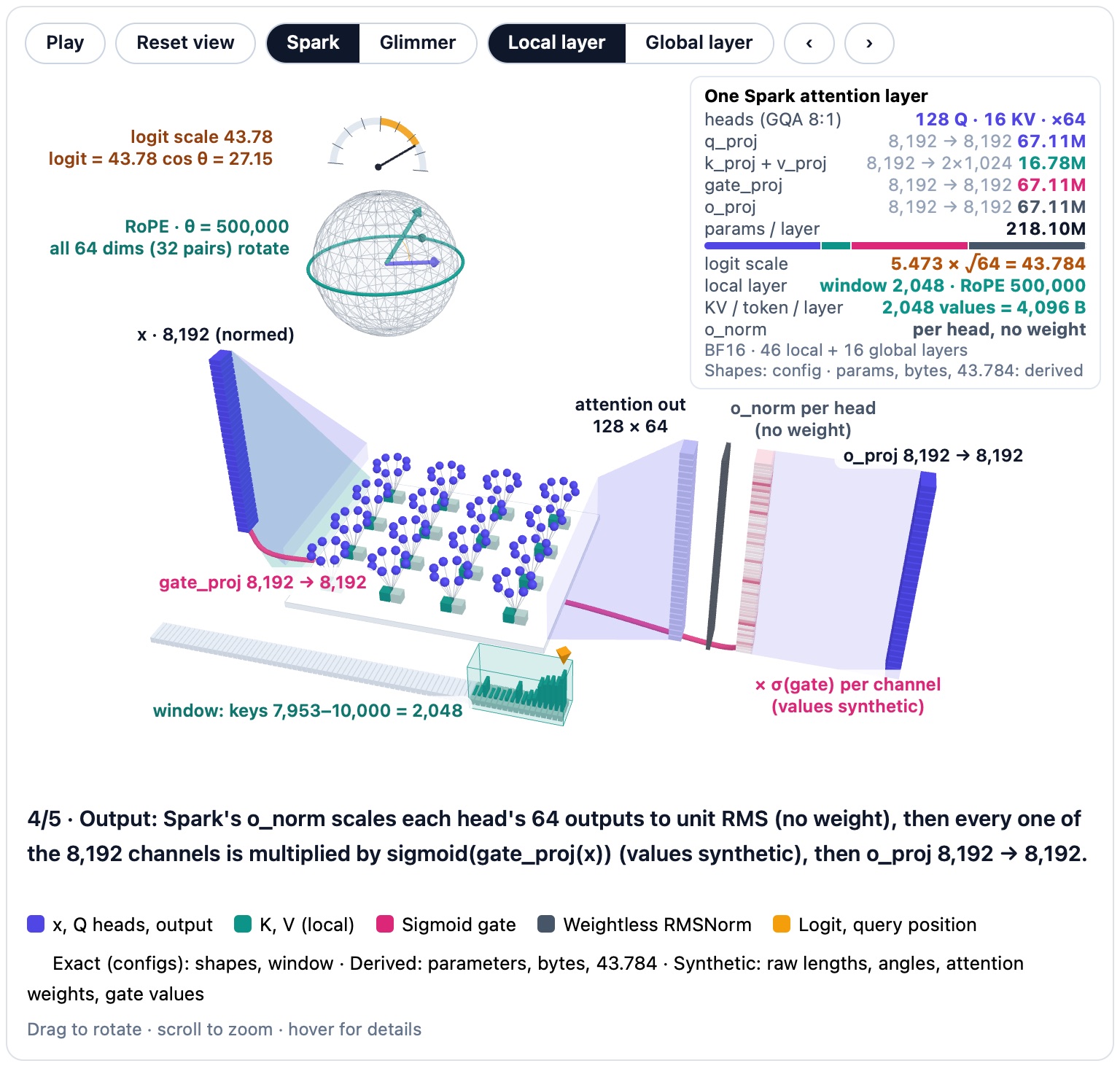
The animation puts §3.1–§3.4 together for one token, Spark’s values first and Glimmer’s in parentheses. Its four beats light up the GQA fan-out (8 query heads per KV head; 16 in Glimmer), the QK-norm with its query multiplier 5.473 (3.87), the RoPE step that only local layers take while global layers bypass it, and finally the whole path, with Spark’s o_norm and the sigmoid gate before o_proj. The three cards underneath repeat the logit bound, the cache per token and the parameter count.

One Muse attention layer for a single token: GQA with 8 (Glimmer 16) query heads per KV head, a weightless per-head QK-norm whose fixed query scale makes every logit 43.784 × cos θ in both models (θ the angle between query and key), RoPE on local layers only, and a per-channel sigmoid gate before o_proj, with Spark adding a weightless per-head output norm; the shapes come from config.json, while the shared 43.784, the cache sizes and the parameter counts are our arithmetic. Open the full-size SVG.

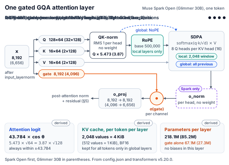
The 3D model below takes the same layer apart in five beats: the GQA shapes, the QK-norm and its single logit scale, the local or global read, the gate (with Spark’s o_norm), and what one token leaves in the cache. Switch between Spark and Glimmer to watch the query heads regroup from 8 to 16 per KV head. Switch between Local and Global to trade the RoPE dial and the 2,048-token window band for a NoPE label and a key row of all previous tokens. In the QK-norm beat the normalized vectors land on a sphere of fixed radius under a “logit scale 43.78” dial: the fixed logit multiplier of §3.2, which this section’s headings call the temperature (strictly an inverse temperature). In the gate beat a strip of per-channel values multiplies the attention output. Shapes, parameter counts and byte counts are exact; attention weights and gate values are synthetic.

Switch Spark and Glimmer to watch the query heads regroup from 8 to 16 per KV head, switch Local and Global to trade the RoPE dial and the 2,048-key window for NoPE and all previous keys, and step through the five beats with ‹ › or Play; shapes are exact, parameter counts, cache bytes and the 43.784 logit scale are derived from the configs, while raw vector lengths, angles, attention weights and gate values are synthetic.

Implementation notes

• The switch: position_embeddings=position_embeddings if self.config.layer_rope_theta[i] else None in MuseSparkTextModel.forward, and if position_embeddings is not None: before apply_rotary_pos_emb in the attention. Only the truthiness of layer_rope_theta matters: one rotary_emb built from rope_parameters["rope_theta"] serves every RoPE layer, so in v5.20.0 the per-layer entries act as an on/off switch. In the released configs every nonzero entry is 500,000, the global value, which llama.cpp’s Spark converter asserts: assert all(t in (0, theta) for t in hparams["layer_rope_theta"]).
• Masks: the model builds create_causal_mask and create_sliding_window_causal_mask once and picks one per layer from layer_types. The sliding mask is kv_idx > q_idx - sliding_window combined with kv_idx <= q_idx (masking_utils.py); the flash backend gets window_size = (sliding_window - 1, sliding_window - 1); the sliding cache keeps “the last self.sliding_window - 1 tokens” between steps.
• RoPE layout: Transformers pairs dimension $j$ with $j + d/2$ (rotate_half); llama.cpp pairs adjacent dimensions, and its converters un-permute the Q/K weight rows to match. Its graphs rotate only when use_rope = hparams.is_swa(il), with the base pinned to the trained value, so --rope-freq-base should not affect Muse (our reading).
• TorchTitan’s Spark attention (model.py) supports a Llama 4-style temperature on global layers, (log((positions + 1) / floor_scale) * query_scale + 1).clamp_min(1.0), but the 816B flavor sets both knobs to None; that flavor’s global_attention_layers=set(range(1, num_layers, 4)) is again 1, 5, …, 61.
• By Mistral’s argument that k windowed layers move information up to k × W tokens (arXiv 2310.06825), the local stack alone reaches 46 × 2,047 = 94,162 tokens in Spark and 39 × 2,047 = 79,833 in Glimmer (derived). Direct long-range reads come from the global layers.

3.5 What Glimmer tried and dropped: MLA in global layers

Global layers hold the only cache that grows with context, so they are the natural place to compress further, and Glimmer’s team tried. The report’s “Design for on-device efficiency” section continues: “we evaluated a simplified Multi-Head Latent Attention (MLA) variant … in global layers by projecting a single joint key-value vector. We tested two configurations: matching either the baseline’s head count (halving KV cache size) or its total KV footprint (doubling head count). Both underperformed standard Grouped Query Attention (GQA) … on long-context benchmarks such as RULER …, leading us to retain GQA.”

MLA, from DeepSeek-V2, caches one compressed latent per token per layer (“low-rank key-value joint compression”) and rebuilds each head’s keys and values from it; the GLM-5.3 post, §3 walks through it. Standard MLA also carries a separate RoPE key, because a position-dependent rotation would block the decode-time trick of folding the key up-projection into the query (§3.3 of that post). Muse’s global layers have no RoPE, so that part would be unnecessary; our guess is that this is part of what “simplified” means. Muse’s per-head QK-norm raises a similar folding question, since normalizing each re-expanded key is not a linear operation.

The benchmark the report names, RULER, is a synthetic long-context suite of retrieval, multi-hop tracing and aggregation tasks. Our arithmetic gives the scale of what was at stake. A Glimmer global layer caches 512 values per token, so the head-count-matched variant would cache about 256. At 131,072 tokens the 13 global layers hold 1.625 GiB, and halving them would save about 0.81 GiB (derived): real, but modest inside a 32 GB envelope. Global layers are the only ones that read past 2,047 tokens directly, so they carry long-range retrieval, and in this ablation that is where compression cost quality. Spark keeps the same GQA design, with 16 KV heads.

Attention is where the two models are nearly identical. §4 turns to the block where they differ most.

---

4. Spark Open’s MoE: 256 Experts in a 4,096-Wide Latent

Where Glimmer has one dense FFN per layer, Spark has an MoE layer in all 62 decoder blocks. The headline numbers are familiar: 256 routed experts, 8 per token, the same pair DeepSeek-V3 uses. What is new is where the experts live. A router scores the token’s full 8,192-number vector, a projection squeezes the vector to 4,096 numbers, the 8 chosen experts work entirely at that width, and a second projection widens the result back. The Transformers code says the block “pools” and “unpools”; llama.cpp and NVIDIA call the structure a latent MoE. (“Latent” here is the pooled 4,096-wide space the experts work in; it is unrelated to the compressed KV latent of MLA in §3.5.) This section takes the block apart in order and ends with the question the Glimmer report answers: why the small model has no experts at all.

4.1 The layer in numbers

How big is one MoE layer, and how much of it does a token touch? It holds 12.95B parameters, and a token uses 471.87M of them, 3.6% (derived). An MoE layer replaces one large feed-forward network with many small ones, the experts, plus a router that sends each token to a few of them; the GLM-5.3 post (§4) walks through the basics. The table lists Spark’s sizes with their keys in config.json (from mlx-community’s public MLX conversion; the Transformers defaults match) and our parameter counts.

Per decoder block	Value	Key or formula
Routed experts	256	num_local_experts
Experts per token	8 (top-8)	num_experts_per_tok
Shared experts	0	num_shared_experts (Transformers ignores it; §4.5)
Blocks with an MoE	all 62	mlp_layer_types = 62 × "sparse"
Router input width	8,192	hidden_size
Latent width (every expert’s input and output)	4,096	moe_hidden_size
Expert (SwiGLU)	4,096 → 2 × 4,096 → 4,096	moe_intermediate_size = 4,096
Parameters per expert (derived)	50,331,648	$3 \times 4{,}096 \times 4{,}096$
All 256 experts (derived)	12,884,901,888	$256 \times 50{,}331{,}648$
Router, two projections, two norms (derived)	69,214,208	$256 \times 8{,}192 + 2 \times 8{,}192 \times 4{,}096 + 2 \times 4{,}096$
MoE total (derived)	12,954,116,096 (12.95B)
Active per token (derived)	471,867,392 (471.87M), 3.64%	8 experts + router + projections + norms
All 62 blocks (derived)	803.16B total, 29.26B active	98.3% and 68.4% of the 816.68B / 42.78B decoder-block counts

One comparison puts the table in proportion (derived). Glimmer’s dense SwiGLU (6,656 → 19,968 → 6,656) has 398.72M parameters, 0.99× the 402.65M in Spark’s 8 active experts. Counting the router, the two projections and the norms as well, Spark’s MoE uses 471.87M parameters per token, 1.18× Glimmer’s FFN. So the two models spend similar FFN effort on each token, but per layer Spark keeps 32.5× as many FFN weights on the shelf (12.95B against 398.72M). §2.3 places these numbers in the full parameter breakdown.

Where the numbers come from

• The docstring of moe_hidden_size reads: “Width the MoE block pools hidden_size down to before the routed experts, and unpools from afterwards. The experts run entirely at this width.” The model card lists “Number of Experts: 256” and “Experts Activated per Token: 8 (top-k routing)”.
• The counts leave out each router’s 256-entry e_score_correction_bias, a buffer rather than a parameter (§4.2). §2.3 reconciles the 62-block totals, 816,680,173,568 and 42,780,753,920, with the official “816B total / 42B active”.

4.2 The router: sigmoid scores, a bias that only chooses

The router turns a token’s vector into 8 expert indices and 8 weights. It reads $h$, the output of the block’s pre_feedforward_layernorm (a centered RMSNorm, §5.3), at the full 8,192 width, not the latent. In order:

1. Score in FP32. Multiply $h$ by the router matrix $W_r$ (256 × 8,192), both cast to float32.
2. Scale. Multiply the 256 logits by output_multiplier = 0.17678 = $1/\sqrt{32} = 1/\sqrt{8{,}192/256}$. The config docstring describes this field as the scale on the language-model (LM) head’s logits before the soft-cap; the router reuses it. §5.4 discusses the $1/\sqrt{d/256}$ rule and why a router is another read-out it fits (our interpretation).
3. Squash. Apply a sigmoid to each logit on its own, giving $s_i \in (0, 1)$. Unlike a softmax, one expert’s score does not lower another’s.
4. Select. Add a per-expert bias $b_i$ and keep the 8 largest values of $s_i + b_i$. All 256 experts compete in one pool, with no group- or node-limited routing.
5. Weight. Drop the bias, divide the 8 winners’ raw scores by their sum (plus $10^{-15}$), and multiply by routed_scaling_factor = 1.0.

\[s_i = \sigma\!\Big(\tfrac{1}{\sqrt{32}}\,(W_r h)_i\Big),\qquad \mathcal{T} = \operatorname{top8}_i\,(s_i + b_i),\qquad g_i = 1.0 \cdot \frac{s_i}{\sum_{j\in\mathcal{T}} s_j + 10^{-15}}\quad (i \in \mathcal{T})\]

In plain terms, with synthetic numbers: expert 17 has a raw logit of 2.77, which the multiplier turns into 0.49 and the sigmoid into $s = 0.62$; its bias is −0.30, so it competes with 0.32. Expert 90 has a raw logit of −2.29, so $s = 0.40$, and a bias of +0.03, so it competes with 0.43 and takes the last slot ahead of expert 17 despite its lower raw score. If the eight winners’ raw scores are 0.72, 0.64, 0.56, 0.52, 0.48, 0.40, 0.36 and 0.32, they sum to 4.00, and the weights are 0.18, 0.16, 0.14, 0.13, 0.12, 0.10, 0.09 and 0.08; expert 90 gets 0.10. The bias decided who; the raw score decides how much.

Because the scaling factor is 1.0, the weights always sum to 1 (up to the $10^{-15}$), so the experts’ contributions form a convex combination (GLM-5.3 and DeepSeek-V4-Pro multiply theirs by 2.5). The multiplier also flattens the sigmoid by a factor of 5.66 (derived): a raw logit must reach 5.66 to give a score of 0.73.

Why a bias? A router left alone tends to collapse onto a few favorite experts, and the classic fix, an auxiliary loss that penalizes uneven load, costs some of the main objective. DeepSeek-V3, following Wang et al. (arXiv 2408.15664), steers mainly with a bias instead (“the bias term is only used for routing”): after each step it lowers an overloaded expert’s bias by γ and raises an underloaded one’s, with γ = 0.001 for the first 14.3T tokens and 0 for the last 500B. Alongside the bias it keeps only a very small sequence-wise balance loss, with weight 0.0001. The GLM-5.3 post (§4.3) covers the idea.

For Spark, the Transformers code only uses the bias. e_score_correction_bias is an nn.Buffer initialized to zeros: it gets no gradient, is not counted in the 816,680,173,568 parameters, and is saved in FP32. There is no update rule and no auxiliary loss; the forward pass computes only the language-model loss. The update rule is described in the README of TorchTitan’s Muse Spark Open implementation (PyTorch’s training library): “Expert bias is updated from token counts to balance expert usage without an auxiliary loss. Each update has its mean removed and uses coefficient 1e-3.” Its shared MoE code applies, before each optimizer step, with $n_i$ the tokens expert $i$ received and $\bar n$ their mean,

\[\Delta b_i = 10^{-3}\,\operatorname{sign}(\bar n - n_i) \;-\; \frac{1}{256}\sum_{j} 10^{-3}\,\operatorname{sign}(\bar n - n_j).\]

For reinforcement learning (RL), the Miles recipe replays the experts chosen during rollout when it trains (rollout routing replay, §9.3).

Implementation notes: the router in code

• In the modular file, class MuseSparkTopkRouter(MiniMaxM2TopKRouter) rewrites the forward pass but keeps MiniMax-M2’s sigmoid, bias-for-choice and renormalization, and it names its changes: “Different from MiniMaxM2: convert to float32 before linear projection and scale by output multiplier.” and “Different from MiniMaxM2: add topk prob eps and scale by routed scaling factor.” It also moves the bias into the router as nn.Buffer(torch.zeros(self.num_experts)).
• The generated file selects with torch.topk(scores_for_choice, k=self.top_k, dim=-1, sorted=False) on routing_weights + self.e_score_correction_bias, then weights with routing_weights.gather(1, topk_indices). Unlike HF’s DeepSeek-V3 router, there is no topk_group masking.
• _keep_in_fp32_modules_strict lists "mlp.gate.weight" and "e_score_correction_bias", so the router stays FP32 when the rest of the model loads in BF16. The Hub lists 130,039,296 F32 values for the BF16 repo (HF API), exactly $62 \times (256 \times 8{,}192 + 256)$ (§2.3).
• llama.cpp folds the multiplier into the router weight at conversion (“Fold it into the weight to keep a plain matmul”) and clamps the renormalization sum at $\ge 6.1035 \times 10^{-5}$ instead of adding $10^{-15}$. TorchTitan keeps a separate router_logit_multiplier of $1/\sqrt{32}$; Transformers reuses one field.

4.3 Pool, compute, unpool

The router decides who; the rest of the block computes. For $T$ tokens, with $h$ of shape [T, 8,192], MuseSparkMoE.forward runs:

1. Pool. pre_expert_proj, a bias-free 8,192 → 4,096 linear layer shared by all experts, maps each token to 4,096 numbers, once per token rather than once per expert.
2. Normalize. pre_expert_norm, a centered RMSNorm over the 4,096 numbers (§4.4), gives the latent vector $z$.
3. Dispatch. Each token’s $z$ goes to its 8 experts.
4. Experts. Expert $i$ computes $E_i(z) = W_{\text{down}}^{(i)}\big(\mathrm{SiLU}(W_{\text{gate}}^{(i)} z) \odot W_{\text{up}}^{(i)} z\big)$ with three 4,096 × 4,096 matrices.
5. Normalize each output. post_expert_norm, an input-scaled RMSNorm with one 4,096-wide weight shared by all 256 experts, brings each output to unit RMS (§4.4).
6. Combine. Multiply by $g_i$ and sum the 8 outputs into [T, 4,096].
7. Unpool. post_expert_proj, bias-free 4,096 → 8,192. The block then applies post_feedforward_layernorm and the residual gate (§5.2).

\[y = W_{\uparrow} \sum_{i\in\mathcal{T}} g_i\, \mathrm{N}_{\text{post}}\big(E_i(z)\big),\qquad z = \mathrm{N}_{\text{pre}}(W_{\downarrow} h),\qquad W_{\downarrow} \in \mathbb{R}^{4096\times 8192},\ \ W_{\uparrow} \in \mathbb{R}^{8192\times 4096}\]

Inside the block, only the router and the two projections touch the 8,192 width. Every expert reads and writes 4,096-number vectors, and the expert-parallel exchange between GPUs moves 4,096-number vectors too.

Why squeeze? In a standard MoE, an expert’s input and output sit at the model width, so each of its three matrices has one side of 8,192. Pooling halves that side, with three effects (the arithmetic is ours):

• Wider experts at the same size. An expert with 50.3M parameters can be 4,096 wide inside instead of 2,048, so the 8 experts give each token 8 × 4,096 = 32,768 hidden SwiGLU units instead of 16,384. The LatentMoE paper calls this the “effective nonlinear budget per token”: the number of active experts times their intermediate width ($U_{\text{eff}} \propto K \cdot m$ in its notation).
• Half the traffic. With expert parallelism (EP) the experts live on different GPUs, and each token’s vector travels to its experts’ GPUs (dispatch) and back (combine) in an all-to-all exchange. Spark sends the latent: one BF16 copy per (token, expert) pair, as HF’s dispatcher sends it, is $8 \times 4{,}096 \times 2$ B = 64 KiB each way, so 128 KiB per token per layer and 7.75 MiB across 62 layers, half of what 8,192-wide rows need. Systems that send 8-bit floating-point (FP8) values or deduplicate per node move fewer bytes, but the factor of 2 holds.
• The price. The two projections hold $2 \times 8{,}192 \times 4{,}096 = 67{,}108{,}864$ parameters per layer, all active: 14.2% of the block’s active FFN parameters and 134 MFLOP per token per layer. And the experts see the token only through a learned 4,096-dimensional projection. LatentMoE reports that model quality holds for compression ratios up to 4 when the expert count is multiplied by the same factor; in its ablation on a 16B-total model compressed by 4, leaving the expert count unchanged “leads to significant quality degradation”. Spark compresses by 2 and keeps 256 experts, a combination the paper does not test.

How much does that buy? The table compares Spark with two designs that do not exist, computed from the same config. Write $E$ = 256 for the expert count, $k$ = 8 for the experts per token and $m$ = 4,096 for the expert’s intermediate width. Design A keeps $E$, $k$ and $m$ but runs the experts at the full 8,192 width; design B keeps the per-expert size and halves $m$ instead.

Per layer unless noted (derived; A and B are not real models)	Spark Open (latent 4,096)	A: no pooling, same $E$, $k$, $m$	B: no pooling, same expert size
Expert shape	4,096 → 2 × 4,096 → 4,096	8,192 → 2 × 4,096 → 8,192	8,192 → 2 × 2,048 → 8,192
Parameters per expert	50.3M	100.7M	50.3M
All 256 experts	12.88B	25.77B	12.88B
Active MoE parameters per token	471.9M	807.4M	404.8M
MoE FLOPs per token ($2 \times$ active)	943.7 MFLOP	1,614.8 MFLOP	809.5 MFLOP
All-to-all per token (BF16, both ways)	128 KiB	256 KiB	256 KiB
Hidden SwiGLU units per token ($k \times m$)	32,768	32,768	16,384
Experts, 62 layers: total / active	798.9B / 24.96B	1,597.7B / 49.93B	798.9B / 24.96B
Decoder blocks, 62 layers: total / active	816.68B / 42.78B	1,611.38B / 63.58B	812.52B / 38.62B

Against A, pooling halves every per-expert cost and turns a 1.61T-parameter design into the 816.68B model, with 42.78B instead of 63.58B active. Against B, a conventional MoE of the same total size, Spark has the same expert parameters and expert FLOPs (the whole MoE costs 943.7 against 809.5 MFLOP because of the projections), twice the hidden width per token and half the traffic, and pays 4.16B extra parameters, all active.

The pattern has a paper. NVIDIA’s LatentMoE (January 2026) makes the same three choices: routing weights “computed from the original token”, experts that operate “entirely within the latent space”, and dispatch in the latent space, which “reduces the communication volume by a factor of α”, the compression ratio $\alpha = d/\ell$ of model width to latent width. Its abstract says the design “has been adopted by the flagship Nemotron-3 Super and Ultra models” (Nemotron 3, arXiv 2512.20856; Nemotron 3 Super, arXiv 2604.12374). The two spend the savings differently. LatentMoE multiplies the expert count by α and, in its default variant, the top-k too, keeping per-token cost constant while adding expert combinations; it adopts α = 4. Spark uses α = 2 and keeps $E = 256$, $k = 8$, DeepSeek-V3’s numbers. Our interpretation is that Spark banks the savings, as a cheaper block than A or a wider expert than B. LatentMoE also routes with a softmax, keeps shared experts at full width and has no norms in its formulas.

The animation follows one token through the block, using the synthetic router numbers from §4.2. Watch the width: 8,192 at the router and the two projections, 4,096 wherever an expert is involved, and one shared norm that every chosen expert’s output passes before its weight applies. The last beat adds a panel with the per-layer numbers of the latent design and of design A.

Spark Open's router reads the full 8,192-wide token, but the 8 experts it picks out of 256 run entirely in a 4,096-wide latent between two projections, followed by one shared post-expert norm, which halves each expert's size and the all-to-all traffic compared with experts at full width (counterfactual, derived); router scores and weights are synthetic. Open the full-size SVG.

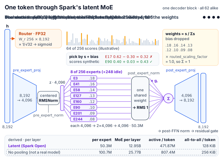
The 3D model shows the same block, with the 256 experts as a 16 × 16 grid of towers. Step through the five beats, then turn the bias off: the winners change, while the weights still come from the unbiased scores. Switch to No pooling (design A) to watch every expert double and the experts of 62 layers grow from 798.9B to 1.6T parameters, or to Glimmer to see one dense 6,656 → 19,968 → 6,656 block instead. Counts and shapes are exact; scores, biases and choices are synthetic.

Step through the five beats with ‹ › or Play, turn the bias off to watch the top-8 change while the weights stay on the raw scores, and switch to No pooling or Glimmer to compare sizes; widths are exact, parameter counts and the no-pooling ghosts are derived, router scores, bias, chosen experts and weights are synthetic.

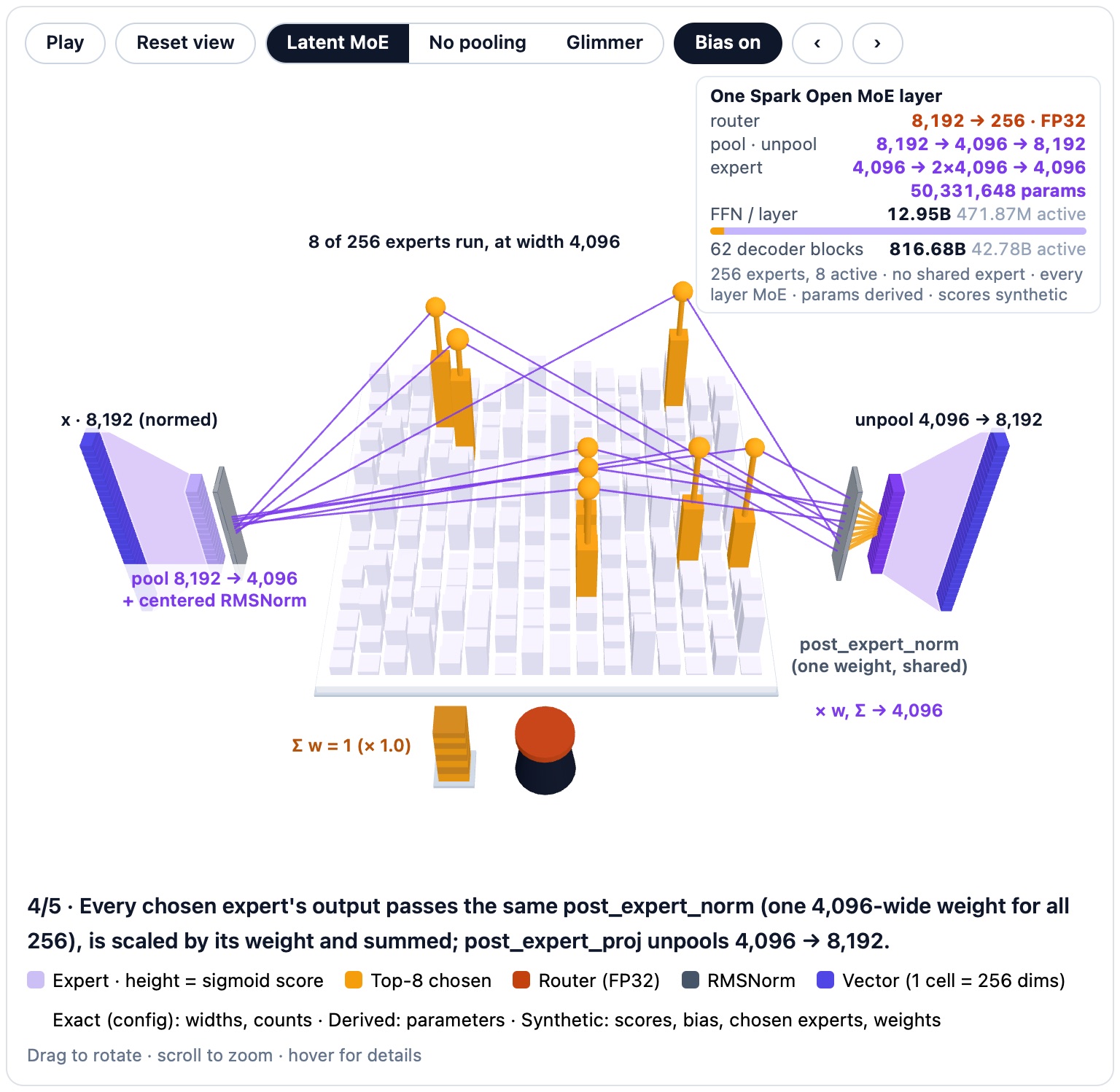
Implementation notes: shapes, storage and parallel plans

• MuseSparkMoE.forward calls the router on the 8,192-wide input first (_, topk_weights, topk_indices = self.gate(hidden_states)), then self.pre_expert_proj, self.pre_expert_norm, self.experts(hidden_states, topk_indices, topk_weights) and self.post_expert_proj.
• MuseSparkExperts(DeepseekV3Experts) sets self.hidden_dim = config.moe_hidden_size and stores the experts as two 3-D tensors, gate_up_proj [256, 8,192, 4,096] (gate rows first) and down_proj [256, 4,096, 4,096], for the grouped-GEMM kernels in integrations/moe.py. The only change to DeepSeek-V3’s expert loop is one line, marked “Different from DeepseekV3 which has no post expert norm”. Read literally, the modular __init__ would allocate at width 8,192 before overriding; the generated file allocates at 4,096, as llama.cpp does.
• MuseSparkTextConfig plans: for EP, split both expert tensors along the expert axis ("grouped_gemm"), move tokens with "ep_dispatch_experts" and replicate the shared norm weight ("replicated_with_grad_allreduce"); for tensor parallelism (TP), mark both projections "rowwise_split_input" (sliced matmul, then all-reduce). The router has no entry, so (our reading) every rank computes it.
• Other names: llama.cpp ffn_latent_down / ffn_latent_up (GGUF key moe_latent_size, comment “The router reads the full stream, not the latent one.”); TorchTitan pooler / unpooler; mlx-lm “The experts run at a compressed width, between the two projections.” Megatron-LM has a --moe-latent-size option. HF’s expert-parallel path runs local experts “with top-1 routing and unit weights; apply routing weights after combine”, which keeps the post-expert norm ahead of the weight.

4.4 Norms inside the MoE

Spark adds two normalizations inside the MoE that neither DeepSeek-V3 nor LatentMoE has. The one after the experts has the visible effect: every chosen expert’s output arrives at the same length, so its share of the sum is exactly its routing weight, and kernels must apply that weight after the norm. Both are 4,096 wide and use the $(1 + w)$ gain convention with $w$ initialized to 0 (§5.3 compares the RMSNorm variants).

pre_expert_norm is a centered RMSNorm (eps $10^{-5}$): normalize, then multiply by $(1 + w)$. Whatever scale pre_expert_proj learns, the experts see a unit-RMS input times a per-channel gain.

post_expert_norm is an input-scaled RMSNorm (eps $10^{-8}$) with the order reversed, scale first and normalize second:

\[\mathrm{N}_{\text{post}}(x) = \frac{x \odot (1 + w)}{\sqrt{\operatorname{mean}\big((x \odot (1+w))^2\big) + 10^{-8}}}\]

The output has RMS 1 whatever $w$ is; the gain only changes which channels dominate the direction. Each layer has one such module, a single 4,096-entry weight applied to every expert’s output: the EP plan replicates it, llama.cpp’s ffn_post_exp_norm has shape {4,096}, and mlx-community’s public weight index holds exactly 62 such tensors, one per layer.

The consequence is clean accounting (the arithmetic is derived, the reading ours). Every chosen expert’s output reaches the weighting step with length $\sqrt{4{,}096} = 64$, so an expert cannot gain influence through larger activations; its share of the sum is exactly $g_i$. With weights summing to 1, the combined latent has RMS at most 1, reaching 1 only when all 8 outputs point the same way. After post_expert_proj, post_feedforward_layernorm, another input-scaled RMSNorm, returns the branch to unit RMS before the residual gate (§5.2).

The nearest relative we found is Megatron-LM’s optional moe_use_norm_before_up_proj, which normalizes once after the combine, not per expert.

The post-expert norm has a systems cost. A normalization erases any scale applied before it, so the routing weight must come after the norm; it cannot be folded into the expert’s activations before the down projection, as DeepSeek-V4’s reference code does (DeepSeek-V4 post, §8.4). It also needs each expert’s whole 4,096-number output: mlx-lm, whose tensor parallelism splits every expert across devices, sums the partial outputs first (“Sum the expert outputs before the post-expert norm”). The SGLang launch blog explains that the order “matters because normalizing the combined output would change the model’s computation,” and lists “per-expert RMS normalization before the route-weighted sum” among what its fused MoE kernel had to support.

4.5 What is not there

Two parts common in MoE models are missing, and the code is explicit about both. A third absence is in the quantized release.

No shared expert. DeepSeek-V3, GLM-5.3 and Llama 4 Maverick (“128 routed experts and a shared expert”, per the Llama 4 blog) run an always-on expert next to the routed ones. Spark’s config.json carries num_shared_experts: 0, but no Transformers or llama.cpp code reads the key and MuseSparkMoE has no shared-expert module; mlx-lm rejects any nonzero value, and TorchTitan raises “Muse Spark MoE does not support shared experts”.

No dense layer. DeepSeek-V3 and GLM-5.3 start with a few dense feed-forward layers, and Llama 4 Maverick alternates dense and MoE layers. Spark’s mlp_layer_types is "sparse" for all 62 blocks, and llama.cpp’s converter asserts it. The dense path still exists: MuseSparkTextMLP (8,192 → 16,384 → 8,192) is built for any layer marked "dense", and intermediate_size: 16384 sits in the config, but neither is used; mlx-community’s weight index has no dense-MLP tensors for the language model. A curiosity (derived): such a layer would have $3 \times 8{,}192 \times 16{,}384 = 402{,}653{,}184$ parameters, exactly the weights of 8 active experts.

No 4-bit weights outside the experts. Meta’s NVFP4 checkpoint quantizes only routed experts, and not all of them. Its quantization_config, as the Hub lists it (HF API), names the experts of layers 0 and 61 in modules_to_not_convert, next to every attention projection, both latent projections, the LM head and the encoders; the SGLang blog confirms “Layers 0 and 61 use BF16 expert weights.” The router stays FP32. §7.4 checks this split against the checkpoint’s dtype counts and sizes the resulting 533 GB checkpoint.

4.6 Why Glimmer is dense

Glimmer was built from the same skeleton, and the Glimmer report says its authors weighed experts and rejected them. Its subsection “Design for on-device efficiency” starts from one constraint: “a strict 32 GB VRAM envelope, which is the practical ceiling for consumer-grade hardware.”

The experiment trained “progressively scaled architectural ladders” comparing “a dense baseline against two Mixture-of-Experts (MoE) designs featuring different routing sparsity (1:8 and 1:16 active experts)”. A ladder is a series of models of growing size trained with one recipe, so that a power law can be fitted and extrapolated to the target budget. Three rules fixed the comparison:

1. Equal memory. Each target model’s parameter count “was chosen such that they can fit into 32 GB VRAM.”
2. Equal compute. Each design’s tokens-per-parameter (TPP) target came from the allocated GPU-hours and its estimated Model FLOP Utilization (MFU): 550 TPP for dense, 2,800 for the 1:8 MoE, 6,000 for the 1:16 MoE.
3. Over-training. “Given our compute budget, all of our ladders operate in over-trained regimes.”

The result: “dense configurations yielded a 2×-2.5× increase in compute efficiency compared to the MoE counterparts. Consequently, we selected a dense 30B parameter design for the architecture.”

In plain terms: at a fixed memory budget the MoE and the dense model hold about the same number of parameters, but the MoE runs only a fraction of them per token, so the same GPU-hours train it on 2,800 / 550 = 5.1× or 6,000 / 550 = 10.9× as many tokens (derived). Those multiples fall short of 8 and 16; our guess is that an MoE’s dense parts and lower MFU eat into the gain. Even with 5–11× more data, the MoE ladders lose. Read off the report’s figure (approximate), the dense ladder sits lowest in both the text and the code panel at every compute level; at the budget it extrapolates to about 0.767 bits per byte (the loss per byte of raw text, which compares across tokenizers; lower is better) on text against about 0.79 for both MoE ladders. We read “compute efficiency” as GPU-hours to reach a given loss.

Our interpretation: when total parameters are capped, an MoE pays for its idle experts in the scarce resource, and what stays active per token is a small model; in an over-trained regime, extra tokens no longer make up for the missing capacity.

Spark answers the same question the other way because it lifts that cap (again our interpretation). It is served from multi-GPU nodes holding 533 GB (NVFP4) to 1.64 TB (BF16) of weights (§7.4), so the comparison that matters is at fixed compute per token, not fixed total parameters. On that axis idle experts cost almost nothing in FLOPs: 42.78B parameters do the work for each token while 816.68B are stored, a 19.1× ratio (derived). Batching spreads the stored weights over many tokens in flight, while FLOPs and all-to-all bytes grow with every token, and those are the costs the latent design trims. As §4.1 showed, the two models end up with similar FFN work per token per layer (Spark’s MoE does 1.18× Glimmer’s, derived) and differ mostly in what they keep on the shelf.

---

5. The Residual Stream: Sandwich Norms and a Norm-Preserving Gate

Every sublayer reads the residual stream and writes something back. Two questions decide how a deep stack behaves: how large can one write be, and how large does the stream become after 104 writes in Glimmer or 124 in Spark (two sublayers per block)? Glimmer answers the first. It wraps each sublayer in a pair of RMSNorms, the Gemma 2 “sandwich”, so every write has a bounded size, but it still adds the writes up, so the stream grows with depth. Spark answers both. It normalizes every branch output to unit RMS and replaces the add with a learned per-channel mix whose coefficients satisfy $\alpha^2 + \beta^2 = 1$. For branch outputs uncorrelated with the stream, that keeps the stream at unit scale from the first decoder block to the last; for correlated ones, it keeps it bounded (§5.2). Both models also fix the two ends of the stream: embeddings enter at unit RMS, and the head rescales and soft-caps the logits.

5.1 Glimmer: sandwich norms

Glimmer bounds every write but lets the stream grow. To see why, start from the two classic layouts. In a pre-norm transformer, a sublayer $f$ reads a normalized copy of the stream and adds its raw output back: $x + f(\mathrm{Norm}(x))$. The input to $f$ is tame; its output is not, and nothing stops one sublayer from writing a vector a hundred times larger than the stream. The original post-norm layout, $\mathrm{Norm}(x + f(x))$, bounds the stream instead, but puts a normalization on the skip path itself. DeepNet (arXiv 2203.00555) frames the choice as one between the “good performance of Post-LN and stable training of Pre-LN.”

The sandwich keeps the skip path an identity and normalizes both ends of the branch. Glimmer’s decoder block, in the order the code runs it:

\[\begin{aligned} h &= x + \mathrm{PostNorm}_1\big(\mathrm{Attn}(\mathrm{PreNorm}_1(x))\big)\\ x' &= h + \mathrm{PostNorm}_2\big(\mathrm{FFN}(\mathrm{PreNorm}_2(h))\big) \end{aligned}\]

That is four RMSNorms per decoder block: input_layernorm, post_attention_layernorm, pre_feedforward_layernorm and post_feedforward_layernorm. Glimmer takes the layout from Gemma 2, whose report (§2, “Post-norm and pre-norm with RMSNorm”) describes it: “To stabilize training, we use RMSNorm … to normalize the input and output of each transformer sub-layer, the attention layer, and the feedforward layer.” Glimmer’s modular file subclasses Gemma 2’s classes directly (MuseGlimmerTextDecoderLayer(Gemma2DecoderLayer), MuseGlimmerTextCenteredRMSNorm(Gemma2RMSNorm)). The placement is older than Gemma 2 and has other names: “Sandwich LayerNorm” in CogView (arXiv 2105.13290) and Peri-LN (arXiv 2502.02732).

All four norms are centered: they normalize, then multiply by $(1 + w)$, so a weight of $w = 0$ means a gain of exactly 1:

\[\mathrm{RMSNorm}(x) = \frac{x}{\sqrt{\tfrac{1}{d}\sum_i x_i^2 + \varepsilon}} \odot (1 + w), \qquad d = 6{,}656 .\]

The pre-norms use $\varepsilon = 10^{-5}$ (rms_norm_eps), the post-norms $10^{-8}$ (post_norm_eps, “used for the post-attention and post-FFN norms (which sit between the sub-layer output and the residual)”). Gemma 2 has one epsilon for all four; §5.3 shows what the split changes.

The post-norm buys a hard bound on each write. Whether the raw attention output has RMS 40 or 0.03, the post-norm rescales it to RMS 1 before the learned gain. That gain, $(1 + w_{\text{post}})$, becomes the sublayer’s per-channel write strength, like LayerScale (arXiv 2103.17239) applied to a normalized vector.

What it leaves unbounded is the stream, because the skip path still adds. Take the idealized case: the embedding enters at RMS 1 (it does, §5.4), every write has RMS 1 (all gains equal to 1), and every write is orthogonal to everything already in the stream. Then the squared RMS grows by 1 per sublayer, and after $\ell$ decoder blocks of two sublayers each,

\[\mathrm{RMS}(x_\ell) = \sqrt{1 + 2\ell}\,: \quad 1.73 \text{ after 1 block},\; 5.20 \text{ after 13},\; 10.25 \text{ after all 52 (derived).}\]

The pre-norms hide the growth from the sublayers, which always see normalized inputs. What shrinks is the weight of each new write: at the top of the stack, a unit write is about a tenth of the stream. Correlation speeds this up; with cosine 0.3 between each write and the stream, the RMS reaches 36.2 after 104 sublayers (derived). The u-µP paper (unit-scaled maximal update parametrization, arXiv 2407.17465, Appendix F) describes the same effect in pre-norm networks: “scale-growth in the skip-stream at initialization, due to the repeated addition of residual connections without subsequent normalization.”

Implementation notes

• MuseGlimmerTextDecoderLayer.forward: residual = hidden_states → input_layernorm → self_attn → post_attention_layernorm → hidden_states = residual + hidden_states, then the same with pre_feedforward_layernorm, mlp, post_feedforward_layernorm. The add runs in the activation dtype.
• 4 weighted norms × 52 blocks + the final norm = 209 vectors, exactly the language model’s norm tensors in the checkpoint index (1,391,104 parameters, derived; the vision tower’s LayerNorms come on top).
• The modular config class deletes three Gemma 2 fields (query_pre_attn_scalar, attn_logit_softcapping and use_bidirectional_attention, each set to AttributeError()); the scaleless QK-norm takes the place of the attention soft-cap (§3.2).
• llama.cpp adds the 1 to the four block-norm weights at conversion (conversion/muse_glimmer.py: “All four layer norms use 1, the final norm uses 0.”), and its graph (muse-glimmer.cpp) hard-codes const float post_norm_eps = 1e-8f;.

5.2 Spark: a residual gate that keeps the norm

Spark’s modular file changes three things in the residual path. The post-attention norm loses its weight. The post-FFN norm becomes “input-scaled” (it multiplies by $1 + w$ first and normalizes last), which guarantees a unit-RMS output (§5.3). And both adds become a MuseSparkResidualGate. The Hugging Face launch blog puts it in one line: “Each block combines its input and its output through a learned residual gate, not through a plain sum.” The whole module, from the modeling file (type hints dropped; the # 0.3 comment is ours):

class MuseSparkResidualGate(nn.Module):
    def __init__(self, config, residual_gate_eps: float = 1e-3):
        super().__init__()
        self.gate = nn.Parameter(torch.empty(config.hidden_size))
        self.temperature = config.residual_gate_temperature   # 0.3
        self.eps = residual_gate_eps

    def forward(self, residual, hidden_states):
        w = self.gate / self.temperature
        beta = torch.sigmoid(w)
        alpha = torch.sqrt(torch.clamp(torch.sigmoid(-w) * (1.0 + beta), min=self.eps))
        return (alpha * residual + beta * hidden_states).to(residual.dtype)

Step by step: the parameter $g$ is a vector of width 8,192, one gate per channel. Divide by the temperature $T = 0.3$ to get $w = g/T$. The branch coefficient is $\beta = \sigma(w)$, the stream coefficient $\alpha = \sqrt{\max(\sigma(-w)(1+\beta),\, 10^{-3})}$, and the output $\alpha \odot x + \beta \odot f$, with $x$ the stream and $f$ the post-normalized sublayer output. Two gates per decoder block make 124 gates and 1,015,808 parameters (derived). The gate never looks at the token: $\alpha$ and $\beta$ depend only on $g$.

Why $\alpha^2 + \beta^2 = 1$. The formula for $\alpha$ is $\sqrt{1 - \beta^2}$ in disguise. Since $\sigma(-w) = 1/(1 + e^{w}) = 1 - \sigma(w) = 1 - \beta$, whenever the clamp is inactive

\[\alpha^2 = \sigma(-w)\,(1 + \beta) = (1 - \beta)(1 + \beta) = 1 - \beta^2 \quad\Longrightarrow\quad \alpha^2 + \beta^2 = 1 .\]

So $(\alpha, \beta) = (\cos\theta, \sin\theta)$ with $\theta = \arcsin\beta$ between 0° and 90°. (Our interpretation of the product form: $1 - \beta^2$ would lose precision as $\beta \to 1$.)

Why that keeps the stream at unit scale. Take one channel $i$, and suppose stream and branch each have unit second moment and are uncorrelated over tokens:

\[\mathbb{E}[\mathrm{out}_i^2] = \alpha_i^2\,\mathbb{E}[x_i^2] + \beta_i^2\,\mathbb{E}[f_i^2] + 2\alpha_i\beta_i\,\mathbb{E}[x_i f_i] = \alpha_i^2 + \beta_i^2 = 1 .\]

The unit-RMS premises are engineered. The branch has unit RMS because both post-norms end with a normalization and no weight after it. The stream starts at unit RMS because embeddings, image features and audio features all pass a weightless RMSNorm (§5.4). Strictly, a norm fixes the RMS over a token’s channels, not each channel’s second moment; but with uncorrelated inputs, $\alpha_i^2 + \beta_i^2 = 1$ makes each channel’s output second moment a weighted average of its two inputs’ (derived), so the mix never inflates it. Geometrically, for orthogonal $x$ and $f$ of equal length, $\cos\theta\, x + \sin\theta\, f$ is $x$ rotated by $\theta$ toward $f$: a step along the circle, not outward.

A four-channel example: $x = [1, -1, 1, -1]$ and $f = [1, 1, -1, -1]$ both have RMS 1 and a zero dot product. A plain add gives $[2, 0, 0, -2]$, RMS 1.414. A gate with $g = 0$ in all four channels ($\beta = 0.5$, $\alpha = 0.866$) gives $[1.366, -0.366, 0.366, -1.366]$, RMS 1.000. At $g = 0.6$ ($\beta = 0.881$, $\alpha = 0.473$) it gives $[1.354, 0.407, -0.407, -1.354]$, RMS 1.000 again. The gate changes which way the stream points, not how long it is. The table lists more gate values; $\theta$ is the angle between the output and $x$ (all derived).

$g$	$\beta$ (branch)	$\alpha$ (stream)	$\alpha^2+\beta^2$	rotation $\theta$
−1.5	0.0067	1.0000	1.000	0.4°
−0.6	0.119	0.993	1.000	6.8°
0	0.500	0.866	1.000	30.0°
+0.6	0.881	0.473	1.000	61.7°
+3.0 (clamped)	0.99995	0.0316	1.0009	88.2°

The clamp. As $\beta \to 1$, $1 - \beta^2$ heads to zero. The code floors $\alpha^2$ at $10^{-3}$, which bites when $\beta > 0.9995$, that is, $g > 2.28$ (derived). From there $\alpha$ stays at $\sqrt{0.001} \approx 0.032$ and $\alpha^2 + \beta^2$ creeps up to at most 1.001, a 0.05% RMS overshoot per gate (derived). Our reading: the floor keeps at least 3.2% of the old stream in every channel and keeps the square root away from zero, where its gradient blows up.

The temperature. Dividing by 0.3 sharpens the sigmoid: $d\beta/dg = \beta(1-\beta)/T$ is 0.83 at $\beta = 0.5$, and $g \in [-1.5, 1.5]$ already spans $\beta$ from 0.0067 to 0.9933 (derived). Under Adam-style updates of roughly fixed size, a step moves the sigmoid’s input $g/T$ 3.3× further than at $T = 1$ (our interpretation).

When branch and stream correlate, the RMS drifts from 1 but stays bounded. For cosine $\rho$ between unit-RMS inputs and one $\theta$ for all channels, one gate gives $\mathrm{RMS}^2 = 1 + \rho\sin 2\theta \le 2$. Over 124 gates with $\beta = 0.5$ and $\rho = 0.3$, the stream settles at RMS 1.65; a plain sum reaches 42.5 (derived). The plain residual fixes the skip coefficient at 1 and lets the scale grow; the gate fixes the scale and lets the skip coefficient shrink.

The figure animates both pictures in four steps. On the left, the plain add steps off the unit circle while the gate turns the stream along it for β = 0.1, 0.5 and 0.9, with the clamp zone near 90°. On the right, the stream’s RMS over depth in the idealized case: $\sqrt{1 + 2\ell}$ for a plain add, 10.25 after Glimmer’s 52 blocks, against a flat 1 for the gate.

Spark’s residual gate mixes the stream and the unit-RMS branch with α² + β² = 1, so it turns the stream along the unit circle instead of lengthening it; the gate points and both depth curves are derived from the formula under an idealized assumption of unit-RMS writes orthogonal to the stream, in which a plain add reaches 10.25 after Glimmer’s 52 blocks while the gate holds the stream at 1. Open the full-size SVG.

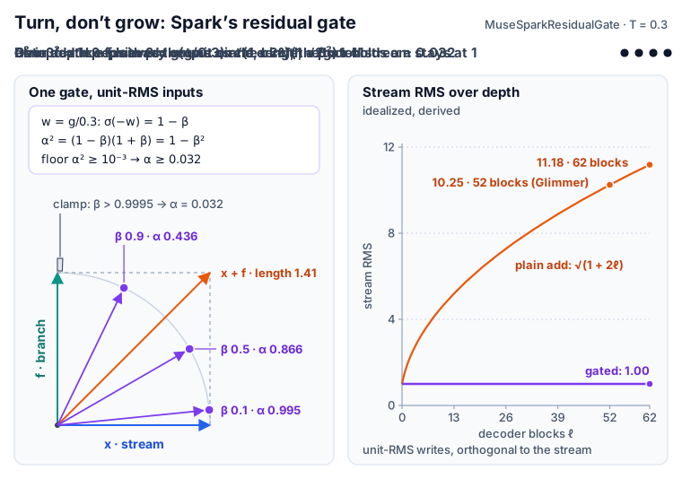
Precision. HF lists both gates in _keep_in_fp32_modules_strict, so the coefficients are computed in FP32 even in a BF16 model; alpha * residual promotes the stream to FP32 for the mix, and .to(residual.dtype) casts it back. A BF16 HF run therefore rounds the stream to BF16 after each of the 124 gates. TorchTitan’s public Muse Spark implementation keeps the stream in FP32 (“Routing scores and the residual stream through the decoder blocks use FP32,” says its README), and so does mlx-lm (h = h.astype(mx.float32)).

Related ideas. The constraint itself is published. Unit Scaling (arXiv 2303.11257) considers the fixed rule $x_{l+1} = \sqrt{1-\tau}\, x_l + \sqrt{\tau}\, f(x_l)$, and u-µP states “the sufficient condition $a_l^2 + b_l^2 = 1$”. Both fix scalar coefficients; Spark learns them per channel. u-µP also shows that for pre-norm networks such scalar weighting is equivalent to a plain residual with rescaled branches, so our reading is that Spark’s additions are the per-channel freedom and a stream kept near unit scale. nGPT, the normalized Transformer (arXiv 2410.01131), also learns per-channel step sizes but renormalizes the stream after every update; Spark does not, and with unit-RMS inputs it does not have to (our reading). On this blog, mHC, manifold-constrained hyper-connections (GLM-5.3 §8.6, DeepSeek-V4 §7), attacks the same problem the other way, with four lanes and a doubly stochastic mixer that cannot amplify the signal and keeps an identity path. Spark keeps one stream and trades the identity skip ($\alpha < 1$) for a fixed scale.

Implementation notes

• MuseSparkTextDecoderLayer.forward: input_layernorm → self_attn → post_attention_layernorm (weightless, ε 1e-8) → post_attention_residual_gate(residual, hidden_states), then pre_feedforward_layernorm → mlp (§4) → post_feedforward_layernorm (input-scaled, ε 1e-8) → post_feedforward_residual_gate.
• residual_gate_temperature: 0.3 is in the config.json of mlx-community’s public MLX conversion, and the code default matches. The 1e-3 floor is a constructor default, not a config field.
• llama.cpp’s converter (conversion/muse_spark.py) precomputes the coefficients (“Norm preserving residual gate: alpha scales the stream, beta the branch, with alpha^2 + beta^2 = 1”, RESIDUAL_GATE_EPS = 1e-3), so its graph only multiplies and adds. mlx-lm does the same in residual_gate_coefficients.
• TorchTitan calls the module MuseSparkNormPreservingResidualConnection; its from-scratch init sets $\beta = 1/(2(\ell+1))$, 0.5 in block 0 down to 0.0081 in block 61. HF’s _init_weights draws $g \sim \mathcal{N}(0, 0.02^2)$, so $\beta \approx 0.5$ everywhere.

5.3 The RMSNorm zoo

Both models together use four kinds of RMSNorm: weightless, centered with a $(1+w)$ gain, Spark’s input-scaled, and a final norm with an absolute gain. The table lists every norm in the order a token meets it; the ε column holds for both models.

Norm (module)	Where	Glimmer	Spark	ε
embed_tokens.embed_norm	after the token lookup (Spark: also audio features)	weightless	weightless	1e-5
perception_emb_norm	after the vision projection	weightless	weightless	1e-5
input_layernorm	before attention	centered	centered	1e-5
self_attn.qk_norm	queries and keys, per head (128 wide in Glimmer, 64 in Spark)	weightless	weightless	1e-5
self_attn.o_norm	attention output, per head (64 wide)	none	weightless	1e-5
post_attention_layernorm	after attention	centered	weightless	1e-8
pre_feedforward_layernorm	before the FFN / MoE	centered	centered	1e-5
mlp.pre_expert_norm	after pooling 8,192 → 4,096	none	centered (4,096)	1e-5
mlp.experts.post_expert_norm	each expert’s output; one weight shared by all 256 experts	none	input-scaled (4,096)	1e-8
post_feedforward_layernorm	after the FFN / MoE	centered	input-scaled	1e-8
norm (final)	before lm_head	absolute gain	absolute gain	1e-5

By our count, Glimmer carries 209 norm weight vectors and Spark 311 (five per decoder block plus the final norm, 2,039,808 parameters; derived). §3.3 covers o_norm, §4.4 the expert norms, and §6 the encoders’ own norms.

Three ways to apply a gain. A weightless norm only divides by the RMS. A centered norm normalizes, then multiplies by $(1+w)$, so the weight sets the output’s size per channel. The input-scaled norm reverses the order: scale by $(1+w)$, then normalize. Its output always has RMS 1; the weight only changes the direction. Take $m = [3, 1]$ and $w = [1, 0]$. Centered: $[1.342, 0.447] \odot [2, 1] = [2.683, 0.447]$, RMS 1.92. Input-scaled: $[6, 1] / 4.301 = [1.395, 0.233]$, RMS 1.00. Our reading: Spark uses the input-scaled form where it needs a unit-RMS vector but still wants a learned channel shape: right before the post-FFN gate, and on each expert’s output right before its routing weight (§4.4).

Two epsilons. An RMSNorm outputs RMS $\sqrt{\mathrm{ms}/(\mathrm{ms}+\varepsilon)}$ for input mean square ms. It still reaches 0.99 for input RMS down to 0.022 with $\varepsilon = 10^{-5}$, and down to 0.0007 with $10^{-8}$ (derived). The post-norms thus deliver unit-RMS writes from branch outputs about 32× smaller. For Spark that protects the gate’s unit-RMS premise (our interpretation); the price is that a near-zero branch output is blown up to full size.

Gain rounding. In a BF16 run, Spark’s port rounds each $(1+w)$ gain to BF16 before applying it, as TorchTitan and mlx-lm do; Glimmer’s port forms the gain in FP32. The implementation notes below trace the cast.

The final norm has an absolute weight that starts at ones. The llama.cpp converter: “Block norms hold a delta around one; the output norm holds an absolute gain.”

The 3D model below adds three things to the animation: β buttons that run up to the clamp (β ≈ 1), with energy bars that set $\alpha^2 + \beta^2$ against $

x + f

^2 = 2$; tiles on Spark’s depth bars that show β varying by channel and layer; and, in the last beat, every norm around a sublayer with its variant and ε, with a Spark Open

Glimmer toggle. The gate formula, norm types and ε are exact; the depth chart is idealized and the per-channel β tiles are synthetic.

Pick β (or press Play) to watch Glimmer's x + f leave the unit circle while Spark's α·x + β·f stays on it, and switch Spark Open | Glimmer to compare the norms around each sublayer; the gate formula, temperature 0.3, clamp 0.001, norm types and eps are exact, the depth chart is idealized and derived, and the per-channel β tiles are synthetic.

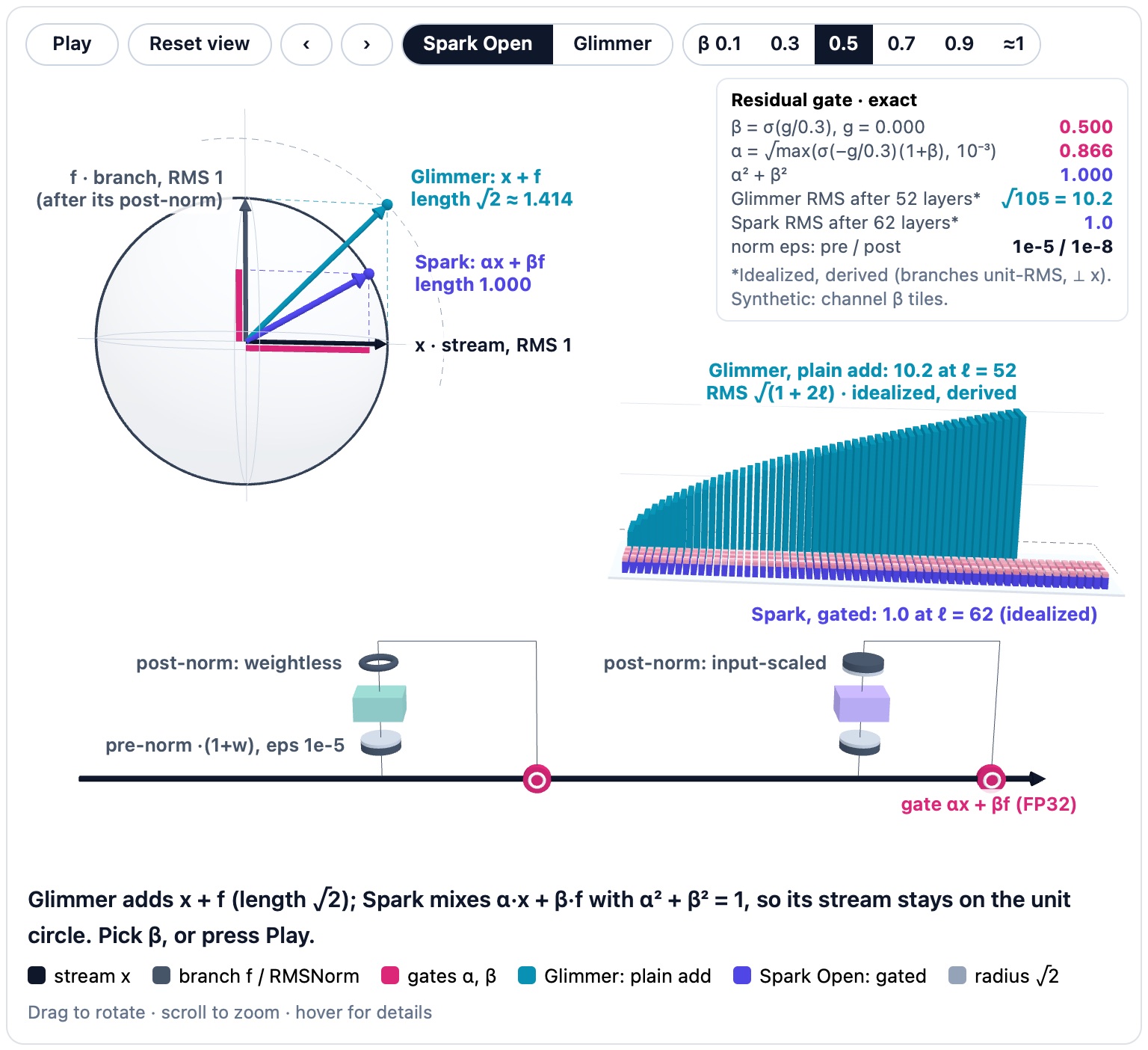
Implementation notes

• Glimmer’s centered norm keeps a Gemma 2 comment: “Llama does x.to(float16) * w whilst MuseGlimmerTextCentered is (x * w).to(float16)”. The multiply runs in FP32 and the result is rounded once. Spark’s copy reads “(x * w).to(bfloat16) instead of x.to(bfloat16) * w”, but one cast moved: Glimmer forms the gain as 1.0 + self.weight.float(), Spark as (1.0 + self.weight).float(). In a BF16 run Spark’s gain is thus rounded to a multiple of $2^{-7} = 0.0078$ in $[1, 2)$ first (derived).
• The input-scaled norm rounds once more: it casts the scaled input back to the input dtype before normalizing, “with fp32->bf16->f32 before norm”.
• Our interpretation: the Spark port copies, on purpose, the BF16 gain rounding of the other public stacks. TorchTitan adds weight + gain_center in the parameter dtype and casts it to the input dtype, and mlx-lm stores (1.0 + weight.astype(mx.float32)).astype(mx.bfloat16).

5.4 Normalized embeddings and a µP-style head

Both ends of the stream are pinned. Every input vector, whatever its modality, enters block 0 at RMS 1, and the head scales the logits by a width-dependent factor and caps them at ±20.

Embeddings. MuseGlimmerTextNormedEmbedding, unchanged in Spark, looks up a row of the 202,048-row table and applies a weightless RMSNorm (ε 1e-5), so every token enters block 0 at RMS 1. The code says the norm “cannot be merged to the embedding matrix, as Dflash implem needs to embed without the norm”. The math would allow folding, since the norm acts on one row at a time (derived); the norm stays separate because the DFlash drafter (§8) shares the target’s table and wants raw rows. HF’s DFlash candidate generator temporarily swaps embed_norm for nn.Identity() to get them.

The other modalities land on the same scale. Image features from the Perception Encoder pass perception_emb_norm, a separate but identical weightless norm; the Glimmer report describes “a single bias-free linear layer followed by parameter-free RMSNorm” (arXiv 2610.24628, “Multimodal input and the perception encoder”). Spark’s audio features leave the audio encoder through its weighted post_proj_norm and then pass the text model’s own embed_norm. Text, image and audio positions all start at unit RMS (§6), the starting condition the argument in §5.2 needs. HF’s Gemma 2, by contrast, multiplies embeddings by $\sqrt{d}$; Muse discards the row’s length, so (our reading) a token’s embedding norm carries no information.

The head. After the final norm comes lm_head, untied from the embedding in both models, and then these four lines (the # 20.0 comment is ours):

logits = logits * self.config.text_config.output_multiplier
logits = logits / self.config.text_config.final_logit_softcapping   # 20.0
logits = torch.tanh(logits)
logits = logits * self.config.text_config.final_logit_softcapping

The final logit is $20\tanh(mz/20)$ for a raw lm_head output $z$. The config docstring defines $m$ as “Equal to 1/sqrt(hidden_size / 256) for the released checkpoint”: $1/\sqrt{26} = 0.19612$ for Glimmer and $1/\sqrt{32} = 0.17678$ for Spark, matching both config values exactly (derived). The soft-cap is Gemma 2’s, $\text{cap} \cdot \tanh(\text{logits}/\text{cap})$, with a cap of 20 instead of 30, and only on the final logits, not on attention.

The cap is nearly linear near zero and flat near ±20: $20\tanh(x/20)$ maps 5 to 4.90, 10 to 9.24, 20 to 15.23 and 40 to 19.28. A final logit of 19 needs $mz = 36.6$, a raw output of 186.8 in Glimmer or 207.2 in Spark. Two tokens’ log-probabilities can never differ by 40 nats or more (all derived).

Why $1/\sqrt{d/256}$. Our interpretation: it is µP’s output multiplier, measured from a base width of 256. In Tensor Programs V (arXiv 2203.03466, Table 9), output weights get initialization variance $1/\text{fan-in}$ and multiplier $1/\sqrt{\text{fan-in}}$, part of the rule set that lets hyperparameters tuned on a narrow model carry over to a wide one. $\sqrt{256/d}$ is that multiplier normalized to 1 at width 256, and TorchTitan’s from-scratch lm_head init uses std $d^{-1/2}$. Two public sources point the same way: the Llama 4 blog’s MetaP, which sets per-layer learning rates and initialization scales meant to transfer across model widths (§3.2), and llama.cpp’s converter, in a contributor’s comment: “MetaP resolves to two scalars / The output multiplier lands here and the attention scale rides on the synthesized QK-norm weights.” The link between MetaP and Muse is our reading of that comment. The second scalar is qk_scale_factor, which fixes the attention temperature at 43.784 (§3.2).

The router borrows the multiplier. Spark’s router multiplies its FP32 logits by the same output_multiplier before the sigmoid (§4.2). The router is another readout from width $d$ to a fixed size, 256 experts, so the same rule fits (our interpretation).

Implementation notes

• Spark applies the text norm to audio literally: self.get_input_embeddings().embed_norm(audio_features) in get_audio_features. The embedding norm is built with config.rms_norm_eps; the class default of 1e-6 is never used.
• No embedding multiplier exists in HF or llama.cpp, and TorchTitan’s 816B flavor sets embedding_multiplier=1.0.
• llama.cpp stores $m$ as the GGUF logit_scale. mlx-lm applies the multiplier and soft-cap in FP32.

---

6. Perception: One Vision Encoder, and an Audio Encoder Without Attention

How do pixels and sound become decoder inputs? For images and video, both models use the same parts in the same order: a 50-layer ViT called the Perception Encoder, a 2 × 2 pixel shuffle that folds each block of four neighbouring patches into one vector, a two-layer adapter, one projection to the text width and a weightless RMSNorm. Spark Open adds an audio tower, a four-stage convolutional pyramid that reads the raw 24 kHz waveform and emits 12.5 tokens per second without any attention. The perception parts are small: 6.45% of Glimmer’s checkpoint and 0.249% of Spark’s (derived).

6.1 The Perception Encoder both models share

Which vision encoder do the two models use? The same architecture: a ViT of 1.85B parameters by our count, from Meta’s Perception Encoder family, with the same sizes and layer schedule in both configs. The Glimmer report introduces it in one paragraph (arXiv 2610.24628, “Multimodal input and the perception encoder”): “we adopt the Perception Encoder which leverages a NaViT-style vision backbone. The encoder is a ~1.8B-parameter ViT-G/14 with 50 layers, width 1536, and patch size 14 that processes images at native resolution using a 448-px reference grid.” The Perception Encoder (arXiv 2504.13181) is Meta’s image and video encoder, trained with CLIP-style contrastive image-text learning; its G-scale vision tower has the same width, depth, MLP width and head count (Table 4 there). NaViT (arXiv 2307.06304) “uses sequence packing during training to process inputs of arbitrary resolutions and aspect ratios.” In Muse’s code that means no fixed input size: the patches of every image in a batch are concatenated into one sequence, and attention stays inside each frame’s segment.

The table shows the tower as both configs define it (Glimmer’s config.json, and for Spark the config.json of mlx-community’s public MLX conversion). The two vision_config blocks agree on every size and on the layer schedule.

Field	Value
Width / layers	1,536 / 50
Attention	16 heads × 96, bidirectional, plain multi-head (no GQA), biased projections
MLP	1,536 → 8,960 → 1,536, exact GELU
Norms	pre-norm LayerNorm with weight and bias (eps 1e-5)
Patch embedding	14 × 14 px × 3 channels × 2 frames = 1,176 inputs → 1,536, no bias
Positions	learned 32 × 32 table, plus 2D RoPE (θ = 10,000) in every layer
Layer schedule	37 window-attention layers, 13 full-attention layers
Parameters (derived)	1,852,639,744

This is a classic ViT, not the decoder scaled down: LayerNorm with biases, no QK-norm, no gates. A still image fills both temporal slots of a patch with the same frame; video fills them with two consecutive frames (§6.2).

Two position signals. The first is a learned table of 32 × 32 vectors, one per patch of the 448-px reference grid, bilinearly resampled to each image’s patch grid (reproducing F.grid_sample with zero padding) and added once after the patch embedding. At 448 px every patch reads exactly one table vector; above 448 px the outermost patches get less than a full vector (weight 0.75 on an edge row at 896 px, derived). The second is 2D RoPE in every layer: each 96-number head splits into a column half and a row half, 24 frequencies per axis, rotated by the patch’s column and row counted from 1. The Perception Encoder paper says why both stay: “We add 2D RoPE to each attention layer to improve extrapolation, keeping the original position embedding.” Glimmer’s config labels this RoPE "default" and Spark’s "axial"; the math is the same, and Transformers v5.20.0 rewrites a saved "default" to "axial" (modeling_rope_utils.py).

Window and full layers. Layers 3, 7, 11, …, 47 and 49 attend over all patches of one frame. The other 37 attend only inside fixed, non-overlapping tiles of 32 × 32 patches (448 × 448 px), laid out from each frame’s top-left corner. These tiles do not slide like the decoder’s local window (§3.4), and no layer attends across two images or two frame pairs of a video. The rule is every fourth layer counted from the bottom plus the last one, so the tail runs 47 full, 48 window, 49 full; the decoder’s three-to-one pattern instead counts back from its top layer (§2.2). The Spark model card describes the scheme as “Sparse attention with factor 4 (every 4th + last layer are full attention)”, so its “sparse” layers are these window layers.

Tiles only matter above 448 px on a side; a smaller image fits in one tile, where both layer types compute the same thing. A 1,920 × 1,080 screenshot is resized to 1,932 × 1,092 px, 138 patches across and 78 down, covered by 15 tiles. The ViT then costs about 51.2 TFLOP instead of 75.4 TFLOP if all 50 layers were full: the window layers save 32% (derived).

One architecture in two releases. The Hugging Face launch blog for Spark Open says that Glimmer “uses an encoder with the same architecture.” The ViT and the adapter have the same shapes in both configs; only vision_projection differs, since it maps to the text width: 6,656 in Glimmer and 8,192 in Spark (derived).

A Spark-specific grid order for the position table. Spark’s Transformers port passes the patch grid to the learned position table as (t, w, h), and TorchTitan’s public Spark flavor likewise gives its vision encoder a Spark-specific order, pos_emb_grid_order="legacy_spark". The layout differs from Glimmer’s only for non-square images; square images read the table the same way, and the 2D RoPE is the same in both. The implementation notes below give the code and a worked example.

Implementation notes

• MuseGlimmerVisionModel.forward (modeling_muse_glimmer.py, v5.20.0) takes packed pixel_values of shape (total patches, 1,176) plus grid_thw, builds per-frame cu_seqlens and the tile permutation, runs the patch embedder and ln_pre, and makes each tile contiguous (hidden_states[window_index, :]). RoPE positions are position_ids.flip(-1) + 1 (“Add 1 because ref implementation’s position offset is 1!”). Layer i gets cu_seqlens_mapping[self.config.layer_types[i]]; afterwards torch.argsort(window_index) restores raster order before ln_post and the pixel shuffle.
• The tile size is not a config key: self.window_size = config.pos_emb_height * config.patch_size = 32 × 14 = 448, tying the tile to the table.
• Per head, columns sit in dims 0–23 and 48–71, rows in 24–47 and 72–95; rotate_half pairs dim i with i + 48, so each rotation plane uses one axis.
• FLOP count (derived, 2 FLOPs per multiply-add): the linear layers cost 2 × 50 × (4 × 1,536² + 2 × 1,536 × 8,960) per patch, and each layer’s attention adds 4 × 1,536 × (segment length)². For the screenshot’s 10,764 patches that is 39.8 TFLOP of linear layers, 9.3 TFLOP of attention in the 13 full layers and 2.1 TFLOP in the 37 window layers, which would cost 26.3 TFLOP as full layers. The patch embedding is left out.
• For still images the 1,176-input patch linear equals a 588-input one with the two temporal halves summed; llama.cpp’s converter folds it that way.
• Spark’s only change to the vision math is an index swap: MuseSparkVisionPatchEmbedder passes grid_thw[:, [0, 2, 1]], that is (t, w, h), to the resampling helper, citing reference code that hands meshgrid(pos_h, pos_w, indexing="xy") to grid_sample. The helper then samples the table on a w-row × h-column grid and assigns the samples in the patches’ h × w raster order. For non-square grids that is a reshape, not a transpose: on a 2 × 3 grid, Glimmer’s top-right patch reads the table near (row 7.5, column 26.2), Spark’s near (15.5, 7.5), in table coordinates 0–31 (derived).
• Glimmer’s vision config gives the ViT a tensor-parallel plan (q, k, v and fc1 column-wise, proj and fc2 row-wise); MuseSparkVisionConfig overrides it with base_model_tp_plan = {}, so under tensor parallelism Spark’s tower is not sharded (our reading: every rank holds a full copy). The adapter and projection keep their column- and row-wise plans in both models.

6.2 From patches to tokens

How does an image become decoder tokens? It is resized once, cut into 14-px patches, run through the ViT, and folded 2 × 2, so each 28 × 28-px cell of the resized image becomes one token: a 448 × 448 image costs 256.

Resize, no tiling. The image processor (Transformers maps muse_spark to MuseGlimmerImageProcessor) resizes each image once, with LANCZOS, to a whole number of 28 × 28-px cells: roughly the image’s own size, rounded to the cell grid whose aspect ratio is closest to the original, and shrunk first if it would exceed 4,096 cells. Pixels are scaled to [−1, 1]. Unlike “dynamic tiling with a thumbnail / global crop”, the report says, “we use a single aspect-ratio-preserving resize to a valid token grid.” One cell becomes one decoder token, so an image costs at most 4,096 tokens: 16,384 patches, or 1,792 × 1,792 px when square (derived).

A 448 × 448 image, step by step:

1. Patchify: 32 × 32 = 1,024 patches of 1,176 numbers.
2. ViT: 50 layers and ln_post give (1,024, 1,536).
3. Pixel shuffle: each 2 × 2 block of neighbouring patches is folded into one vector of 4 × 1,536 = 6,144: (256, 6,144). Nothing is averaged away.
4. Adapter: bias-free fc1 6,144 → 4,096, GELU, fc2 4,096 → 4,096, GELU again: (256, 4,096).
5. Projection: one bias-free linear to the text width, (256, 8,192) in Spark, (256, 6,656) in Glimmer.
6. Weightless RMSNorm: each vector divided by its RMS (eps 1e-5), no learned scale.
7. Scatter: the 256 vectors overwrite 256 <|patch|> placeholders (id 200092) between <|image_start|> and <|image_end|>.

The 14-px patch, 2-frame temporal patch and 2 × 2 merge are the recipe we met in GLM-5.3-Flash’s encoder (GLM-5.3 post, §8.8). The Spark card’s “4096 output dim” matches the adapter’s output width (projector_hidden_size), not the 6,144 after the shuffle or the decoder’s 8,192. The table shows other sizes, derived by running smart_resize and the tile rule:

Input (H × W px)	Resized to	Patch grid	ViT tiles	Decoder tokens
100 × 100	112 × 112	8 × 8	1	16
448 × 448	448 × 448	32 × 32	1	256
1,080 × 1,920	1,092 × 1,932	78 × 138	15	2,691
4,000 × 4,000	1,792 × 1,792	128 × 128	16	4,096 (cap)

Why end with a weightless norm? Our reading: it puts image vectors on the same scale as text. Text embeddings and Spark’s audio features get the same weightless normalization, so every input position starts at RMS 1 (§5.4). In the decoder, image tokens take ordinary consecutive 1-D positions: RoPE in local layers, none in global layers (§3.4). The 2-D layout arrives only through the encoder features and the raster order of the 2 × 2 blocks (our reading).

Video. The default MuseGlimmerVideoProcessor samples 2 frames per second, at most 96 frames spread evenly over the clip, and pairs consecutive sampled frames: each 1,176-number patch holds the same 14 × 14 square from two frames. Each pair (one second of video at the default rate, until a clip passes 48 s) is resized to at most 144 tokens, 252 × 448 px for a 720p or 1080p frame, and gets a text timestamp such as Time: 3.5s (the Hugging Face blog’s example) before its <|video|> placeholders (id 200091). A clip tops out at 48 pairs × 144 = 6,912 visual tokens plus the timestamps (derived), as the deployment docs say: “capped at ~6.9K tokens from about 48 seconds on.” Full attention never spans two pairs, so only the decoder mixes information across them. Both models share this processor, but only Spark’s card lists video as an input; Glimmer’s report says it can ingest video “as a sequence of frames” but “is not explicitly optimized for video.”

The Spark card warns that “very short or low-resolution videos (a few seconds at around 100 px)” may fail and recommends “448 px or more on the short side”. The arithmetic shows how little such a clip leaves the decoder: a 100 × 100 clip becomes 112 × 112 px, 16 tokens per pair, so a 2-second clip yields 32 visual tokens (derived). The default processor shrinks every 16:9 source with 448 px or more on the short side to 252 × 448 per pair.

Parameters. The table counts the vision path from the shapes (derived). Together with the decoder and, for Spark, the audio tower, these counts reconcile with both Hub checkpoint totals (§2.3).

Component (derived)	Formula	Glimmer	Spark
ViT tower	patch 1,806,336 + table 1,572,864 + 2 LNs 6,144 + 50 × 36,985,088	1,852,639,744	same
Adapter	6,144 × 4,096 + 4,096 × 4,096	41,943,040	same
Projection	4,096 × text width	27,262,976	33,554,432
Vision path		1,921,845,760	1,928,137,216

The “1.8B” in the card and the report corresponds to the tower alone (1.853B; our reading). §2.3 places these counts in the whole parameter budget.

Implementation notes

• smart_resize starts from the image’s size in 28-px cells, scales it down to the 4,096-cell cap if needed, tries the floor and ceiling of both sides, and keeps the candidate whose aspect ratio is closest to the input’s; it does not enlarge a small image beyond that rounding. For a square input the floor and ceiling grids tie, and the code keeps whichever comes first in a Python set: 4 × 4 cells (112 px) for a 100 × 100 image (derived by running the function).
• pixel_shuffle ends in hidden_states.view(-1, factor * factor, dim).permute(0, 2, 1).reshape(-1, dim * factor * factor) with factor = 2, so out[o, 4c + s] = x[4o + s, c] for patch s of block o: channel-major, patch-minor. Inside the tower spatial_merge_size stays 1; “the merge is deferred to pixel_shuffle”.
• MuseGlimmerVisionAdapter.forward is self.act(self.fc2(self.act(self.fc1(x)))); get_image_features then applies vision_projection and perception_emb_norm = MuseGlimmerRMSNorm(..., with_scale=False). The forward pass zeroes placeholder ids before the embedding lookup, then calls inputs_embeds.masked_scatter(image_mask, image_embeds).
• The image and video limits in this section are the defaults of the shared processors in Transformers v5.20.0.

6.3 Spark’s audio encoder: 24 kHz to 12.5 Hz with convolutions only

How does Spark turn sound into tokens? One second of 24 kHz audio is 24,000 numbers, and the decoder gets 12.5 vectors for it. Spark closes the gap with one fixed pipeline, which its code describes as “a fully causal convolutional pyramid that maps raw mono 24 kHz audio to one embedding per 1920 samples (80 ms, i.e. 12.5 Hz), already in the text model’s hidden size. It uses no attention and no spectrogram front-end” (modular_muse_spark.py). The feature extractor “only batches, pads and (optionally) truncates”: mono only, 24,000 Hz only, zero-padded on the right to a multiple of 1,920 samples.

Four stages. Each stage first folds p consecutive frames into one (a reshape from (B, T, C) to (B, T/p, p·C), then a linear layer and an RMSNorm), and then refines the shorter sequence with two conv blocks. A block is a depthwise causal convolution over time with kernel 7 (each channel filtered on its own), an RMSNorm, an MLP that widens 4× with GELU, and a residual add, a ConvNeXt-like block in our terms. Stage 0’s “patch” is 16 raw samples, so its linear layer acts as a learned filterbank (our reading). The patch sizes multiply to the samples behind one token:

\[\text{tokens} = \left\lceil \frac{\text{samples}}{16 \times 6 \times 5 \times 4} \right\rceil = \left\lceil \frac{\text{samples}}{1{,}920} \right\rceil, \qquad \frac{1{,}920}{24{,}000\ \text{Hz}} = 80\ \text{ms}.\]

The table follows one stage per row; everything except the patch sizes and widths is derived.

Stage	Patch	Width	Frame rate	Frame length	Frames per token	Parameters
0	16 samples	256	1,500 Hz	0.67 ms	120	1,060,352
1	6 frames	512	250 Hz	4 ms	20	4,996,096
2	5 frames	1,024	50 Hz	20 ms	4	19,429,376
3	4 frames	2,048	12.5 Hz	80 ms	1	75,558,912
Head	RMSNorm → linear → RMSNorm	2,048 → 8,192	12.5 Hz	80 ms	1	16,795,648

The tower holds 117,840,384 parameters (derived). The frame rate falls faster than the width grows, so compute per second of audio is roughly balanced across stages, about 9.9 GFLOP per second for the whole tower (derived). The animation zooms in on one 80 ms token: watch 1,920 samples become 120 stage-0 frames, then 20, 4 and finally one 2,048-wide frame that the head lifts to 8,192. Its third beat previews the causal receptive field explained below.

Spark Open's audio tower folds 16, 6, 5 and then 4 frames per stage, so 1,920 raw 24 kHz samples (80 ms) become one 8,192-wide token through depthwise causal convolutions that see 1.336 s of past audio and none of the future; the waveform is illustrative, and the per-stage rates, frame counts, parameters, receptive field, cache size and compute are derived from the config. Open the full-size SVG.

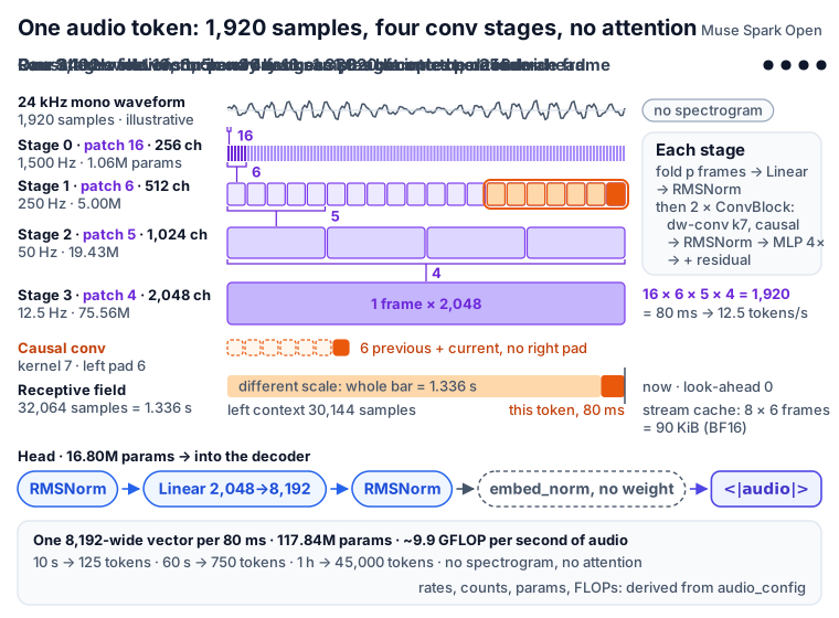
A 60-second clip (derived). 60 s × 24,000 = 1,440,000 samples, already a multiple of 1,920. The shapes run (1, 1,440,000, 1) → (1, 90,000, 256) → (1, 15,000, 512) → (1, 3,000, 1,024) → (1, 750, 2,048) → head (1, 750, 8,192). The 750 vectors pass the text embedding’s weightless embed_norm and overwrite 750 <|audio|> placeholders (id 200038) between <|soft_audio_start|> and <|soft_audio_end|>. Ten seconds give 125 tokens, as the Hugging Face blog says, and an hour 45,000. The tower spends about 0.59 TFLOP on the minute, under 1% of the roughly 64 TFLOP the decoder blocks’ matmuls spend prefilling those 750 tokens (750 × 2 × 42.78B). The tower emits continuous vectors, not codebook entries, and needs no adapter: its own projection maps straight to 8,192, and the config check insists on it because “the audio encoder’s output is scattered directly onto the text embeddings.”

Causal, so it can stream. Every convolution pads 6 frames on the left and none on the right; the conv class and its padding cache are inherited unchanged from Voxtral Realtime (modeling_voxtral_realtime.py). Two convolutions per stage, each reaching 6 frames back, give one token’s receptive field (derived):

\[1{,}920 + 2 \times 6 \times (16 + 96 + 480 + 1{,}920) = 32{,}064\ \text{samples} = 1.336\ \text{s},\]

all of it at or before the token’s own 80 ms, with no look-ahead. With a padding_cache, each convolution keeps its last 6 input frames between chunks, 46,080 values or 90 KiB per stream in BF16 (derived). Because the cache supplies exact left context and patches never straddle a 1,920-sample boundary, feeding 80 ms chunks should reproduce the offline output (our reading).

Implementation notes

• MuseSparkAudioModel.forward: hidden_states = input_values.unsqueeze(-1), four MuseSparkAudioLayers, then self.post_proj_norm(self.proj(self.norm(hidden_states))). A layer is MuseSparkAudioPatchEmbedding (reshape(batch_size, seq_len // self.patch_size, self.patch_size * channels), then self.norm(self.proj(...))) followed by two MuseSparkAudioConvBlocks, each computing MLP(RMSNorm(conv(x))) + x.
• MuseSparkAudioCausalConv1d(VoxtralRealtimeCausalConv1d) uses left_pad = (kernel_size - 1) * dilation + 1 - stride = 6 and groups=hidden_size (depthwise). Audio RMSNorms have learned weights and eps 1e-6; the weightless text embed_norm (eps 1e-5) follows post_proj_norm.
• get_audio_features drops padding-only tokens with num_tokens = (lengths + samples_per_token - 1) // samples_per_token. llama.cpp’s muse-spark-audio.cpp follows the same order and maps “straight into the text hidden size, no adapter”.

---

7. Long Context and Memory Arithmetic

What does a million-token context cost Muse Spark Open, and how much of Glimmer’s 32 GB budget is left once the weights are loaded? The layer schedule from §2.2 does most of the work. Only the 16 global layers keep a cache that grows with context, so one 1M-token sequence needs 64.4 GiB of BF16 cache instead of 248 GiB, and positions need no RoPE scaling at all. What does keep growing is attention arithmetic: past about 164K tokens, Spark spends more FLOPs per token on attention than on all of its weight matrices combined. Unless a source is named, every number here is our arithmetic from the two configs for one sequence, not a measurement.

7.1 A million positions without RoPE scaling

How does Spark reach a million positions? Its config simply declares them, and neither model’s config asks for any RoPE scaling. Spark’s config.json sets max_position_embeddings to 1,048,576, and the model card lists “Context Length | 1M at inference”. Glimmer’s config sets 131,072, which its card writes as “131,072+” and the report as “128K+”; the report’s second mid-training phase extends the window from 32K to 128K (§9.1). Both use the same RoPE block, {"rope_theta": 500000.0, "rope_type": "default"}, with no YaRN or other scaling factor. DeepSeek-V4, by contrast, reaches 1,048,576 positions by stretching a 65,536-token design with YaRN factor 16 (DeepSeek-V4 post, §9.1).

§3.4 explained why Muse can skip that step. A local layer only compares tokens 0 to 2,047 positions apart, however long the document, so its RoPE angles never leave the range it saw in training. A global layer has no positional encoding to extrapolate; position reaches it through the causal mask and the residual stream.

What still changes with length is how thinly a global layer spreads its attention: at 1M, one softmax covers up to 1,048,576 keys. §3.2 showed that QK-norm and the fixed scale keep every logit between −43.784 and +43.784 in both models. How much of that range does a long context need?

In plain terms: take one relevant key and $N$ unrelated keys at logit 0. The relevant key gets half the attention weight once its logit reaches $\ln N$: $\ln 8{,}191 \approx 9.0$ at 8K context and $\ln 1{,}048{,}575 \approx 13.9$ at 1M (derived). Going from 8K to 1M asks a head for 4.85 more logit units, and the 13.9 needed at 1M is still under a third of the ceiling. Our reading: at long context the risk is diluted attention, not unseen positions, and the ceiling leaves room to resist dilution.

Implementation notes

• No scaling anywhere. Both configs use rope_type: default with no original_max_position_embeddings, and the default RoPE init returns attention_factor = 1.0 # Unused in this type of RoPE (modeling_muse_spark.py). §3.4 quotes the line that hands RoPE to local layers only.
• Serving the full window. Meta’s deploy page starts vLLM on NVIDIA with --max-model-len 1048576. For llama.cpp, the same page notes that the context is divided across -np slots, “so long-context agents should use -np 1”.
• Glimmer: Meta’s Glimmer deploy page serves the GGUF with -c 131072 -np 1 and expects a 131,072-token slot. If the file’s context_length metadata is stale, llama.cpp clamps the slot to that smaller value: “No serve flag overrides this.” The page gives a script that rewrites the key to 131072.

7.2 The KV cache, layer by layer

How large is one sequence’s cache? Only the global layers’ share grows with context. §3.1 counted what one token stores in one layer: K and V for every KV head, $2 \times 16 \times 64 = 2{,}048$ values (4 KiB in BF16) for Spark and $2 \times 2 \times 128 = 512$ values (1 KiB) for Glimmer. A local layer keeps at most 2,048 tokens. Only a global layer multiplies its entry by the full context $c$. With $b$ bytes per token per layer:

\[\mathrm{KV}(c) \;=\; \underbrace{n_{\text{global}}\, b\, c}_{\text{grows with context}} \;+\; \underbrace{n_{\text{local}}\, b\, \min(c,\, 2{,}048)}_{\text{capped}}\]

In plain terms (§2.2 previewed these numbers): each new token adds $16 \times 4$ KiB = 64 KiB to Spark’s cache and $13 \times 1$ KiB = 13 KiB to Glimmer’s, instead of 248 KiB and 52 KiB if every layer were global. The capped part is $46 \times 2{,}048 \times 4$ KiB = 368 MiB for Spark and $39 \times 2{,}048 \times 1$ KiB = 78 MiB for Glimmer. The growing part passes it at 5,888 and 6,144 tokens (all derived). Meta’s settings page says the same: “Only the full-attention layers keep a KV cache for the whole context, so KV memory grows with context length on those 16 layers and stays fixed on the rest.”

The animation builds Spark’s figure in four steps: 4 KiB per token per layer, the 46 capped local layers, the 16 growing global layers, and the total next to the dashed all-global outline. Watch the local part shrink from a large share at 8K to a sliver at 1M.

Only Spark’s 16 global layers keep every token, so its BF16 cache grows by 64 KiB per token and reaches 64.4 GiB at 1M tokens, about a quarter of the 248 GiB an all-global design would need, while the capped local part falls from 42% of the cache at 8K to 0.56% (all values derived from the configs; the dashed all-global bars are a counterfactual, and each panel has its own scale). Open the full-size SVG.

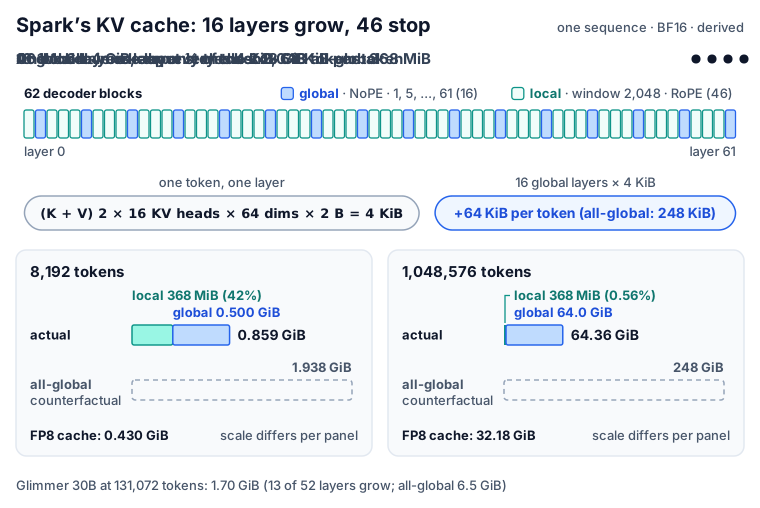
The table splits one sequence’s cache into its growing global part and its capped local part (all derived). The all-global columns are a counterfactual, not a real model. Glimmer’s values in parentheses are beyond its 131,072-token window.

Context (tokens)	Spark global + local, BF16	Spark total, BF16 / FP8	Spark if all-global	Glimmer global + local, BF16	Glimmer total, BF16 / FP8	Glimmer if all-global
8,192	0.500 GiB + 368 MiB	0.859 / 0.430 GiB	1.938 GiB	0.102 GiB + 78 MiB	0.178 / 0.089 GiB	0.406 GiB
32,768	2.000 GiB + 368 MiB	2.359 / 1.180 GiB	7.750 GiB	0.406 GiB + 78 MiB	0.482 / 0.241 GiB	1.625 GiB
131,072	8.000 GiB + 368 MiB	8.359 / 4.180 GiB	31.000 GiB	1.625 GiB + 78 MiB	1.701 / 0.851 GiB	6.500 GiB
262,144	16.000 GiB + 368 MiB	16.359 / 8.180 GiB	62.000 GiB	(3.250 GiB + 78 MiB)	(3.326 / 1.663 GiB)	(13.000 GiB)
1,048,576	64.000 GiB + 368 MiB	64.359 / 32.180 GiB	248.000 GiB	(13.000 GiB + 78 MiB)	(13.076 / 6.538 GiB)	(52.000 GiB)

Three things stand out:

1. The cap matters only at short context. At 8K the local layers hold about 42% of Spark’s cache. At 1M they hold 0.56%.
2. The ratio to all-global falls toward the layer ratio, 16/62 = 0.258 for Spark and 13/52 = 0.25 for Glimmer. At 1M Spark is at 0.260, which the vLLM blog calls “just over ¼ of what all-full attention would need.”
3. On GB300 with TensorRT-LLM, the FP8 column is the one that applies. TensorRT-LLM’s deployment guide requires an FP8 cache there whenever chunked prefill or KV reuse is on, because “for head dimension 64 on SM103, the fused paged-context FMHA kernel exists only for the FP8 KV-cache dtype.” (SM103 is GB300’s GPU architecture.)

Glimmer’s 131,072 row can be checked against a measurement. Meta’s quantization page reports “KV cache and compute buffers | 2.1 GiB” at a full 131,072-token context in llama.cpp, consistent with our 1.70 GiB plus about 0.4 GiB of compute buffers (our interpretation). The page gives the same reason we do: “only a quarter of the layers hold a full-length cache.”

The 3D chart puts both models on one axis from 1K to 1M tokens, Spark in the back row and Glimmer in front. Blue marks global layers, teal local (sliding-window) layers, and outlines the all-global counterfactual. The axis starts in log scale, with the local and global parts side by side at each context, each on the log axis: the teal column stays flat from 2,048 tokens on while the blue one keeps growing. Linear stacks the two parts into one column drawn to scale. Step through the beats, then switch to FP8 to halve every column. The Compute / token view plots the attention FLOPs that §7.3 derives next. Hover any column for its exact value. Glimmer’s row stops at 131,072.

Step through the five beats or switch between KV cache and compute per token, BF16 and FP8, Spark, Glimmer or both, and log scale (local and global parts side by side) or linear scale (stacked to scale), then hover or tap a column for its bytes or FLOPs; every number is exact from the configs or derived, and nothing is synthetic.

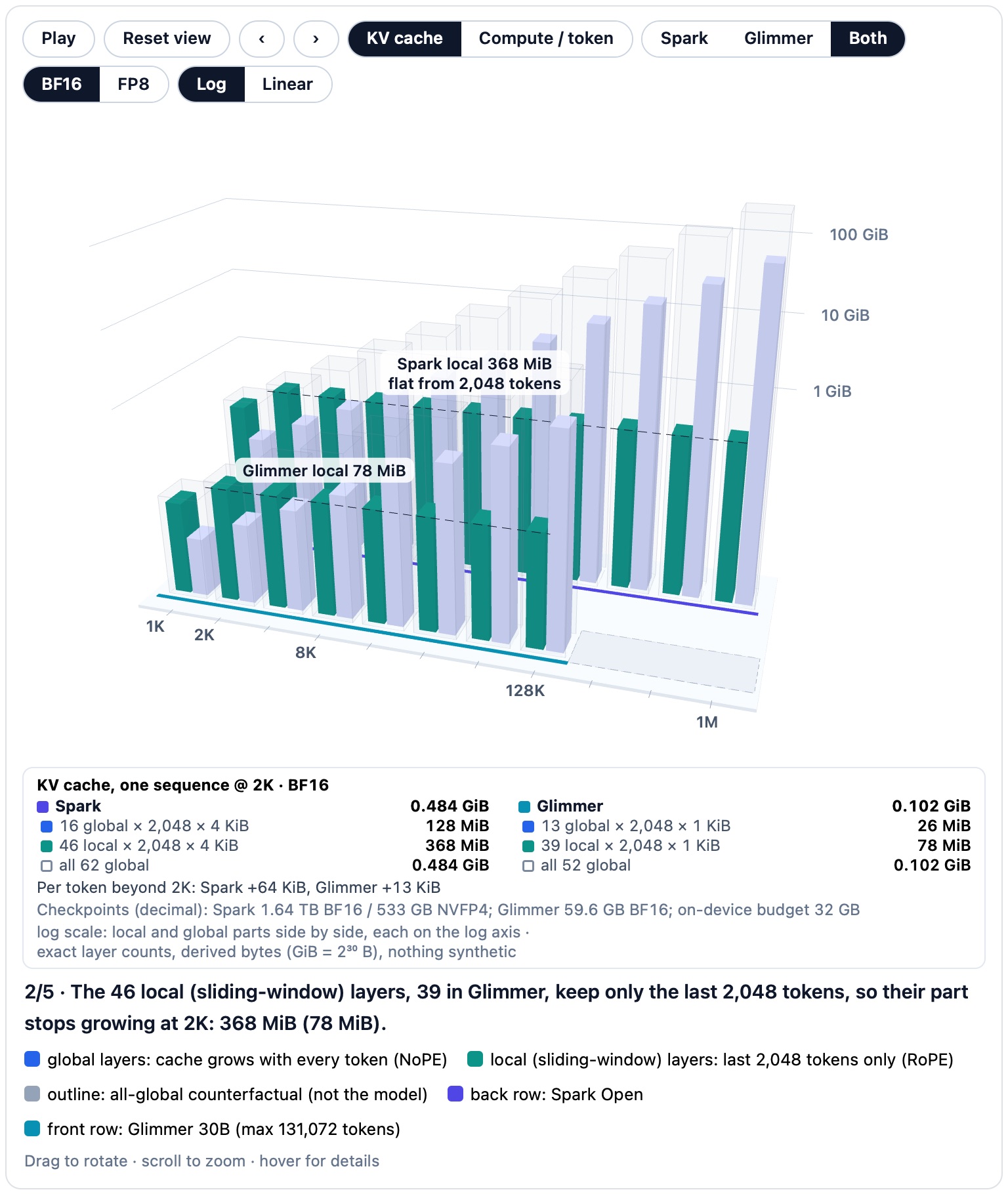
Where the numbers come from

• Config keys: num_key_value_heads 16 / 2, head_dim 64 / 128, sliding_window 2048, and 16 / 13 full_attention entries in layer_types. Bytes: 2 per value in BF16, 1 in FP8, ignoring scale factors.
• The window: Transformers gives each local layer a DynamicSlidingWindowLayer, which keeps “the last self.sliding_window - 1 tokens” (self.keys = full_key_states[:, :, -self.sliding_window + 1 :, :], cache_utils.py). With the incoming token, a local layer sees the current token plus the previous 2,047. Caching 2,047 tokens instead of 2,048 gives Spark 367.8 MiB instead of 368.0 MiB, a negligible difference.
• Not counted: activations, paging overhead and the drafter’s own cache (about 40 MiB, §8.2). GiB = $2^{30}$ bytes, GB = $10^9$ bytes.
• Counterfactual for scale: a DeepSeek-V2-style MLA entry of 576 values per token, a 512-value latent plus a 64-value RoPE key (arXiv 2405.04434), in Spark’s 16 global layers would bring 1M down to 18.4 GiB (derived). For Glimmer that latent is larger than its 512-value GQA entry. §3.5 covers the MLA variant that Glimmer tried and dropped.

7.3 Compute per token

How much arithmetic does one decoded token cost? A fixed price for the weight matrices, plus an attention price that grows with context. The fixed price uses the usual two FLOPs per weight touched, applied to the active decoder parameters (§2.3) plus lm_head:

\[\text{Spark: } 2 \times (42{,}780{,}753{,}920 + 202{,}048 \times 8{,}192) = 88.9\ \text{GFLOP}, \qquad \text{Glimmer: } 2 \times (25{,}165{,}111{,}296 + 202{,}048 \times 6{,}656) = 53.0\ \text{GFLOP}\]

For attention, every query head scores every visible key and adds that key’s value into its output: two length-$d$ dot products, so $4 \times n_q \times d$ FLOPs per key per layer. That is 32,768 for Spark and 16,384 for Glimmer. GQA does not reduce this cost. Shared KV heads save bytes, but every query head still scores every key. For Spark at $c \ge 2{,}048$:

\[A(c) \;=\; 32{,}768 \times \big(16\,c + 46 \times 2{,}048\big) \;=\; 524{,}288\,c \;+\; 3.087 \times 10^{9}\ \text{FLOP}\]

The table gives attention FLOPs per decoded token and their share of the total (derived). Softmax, norms and the gate’s element-wise multiply are left out; the gate’s projection is part of the fixed price.

Context (tokens)	Spark attention	Spark share	Spark if all-global	Glimmer attention	Glimmer share
8,192	7.4 GFLOP	7.7%	16.6 GFLOP	3.1 GFLOP	5.4%
32,768	20.3 GFLOP	18.6%	66.6 GFLOP	8.3 GFLOP	13.5%
131,072	71.8 GFLOP	44.7%	266.3 GFLOP	29.2 GFLOP	35.5%
1,048,576	552.8 GFLOP	86.2%	2,130.3 GFLOP	—	—

Attention overtakes the weight matrices where $A(c) = 88.87 \times 10^9$:

\[c^{*} \;=\; \frac{88.87 \times 10^{9} - 3.087 \times 10^{9}}{524{,}288} \;\approx\; 163{,}600 \ \text{tokens} \;\approx\; 164\text{K}\]

For Glimmer, $212{,}992\,c + 1.309 \times 10^{9} = 53.02 \times 10^{9}$ gives about 242,800 tokens, beyond its window, so across Glimmer’s trained range the weight matrices always dominate (derived).

In plain terms: at 1M, Spark spends 552.8 GFLOP per token on attention, 549.8 of them in the 16 global layers, against 88.9 GFLOP for everything else. Prefilling a 1M-token prompt costs about $3.85 \times 10^{17}$ FLOP, three-quarters of it attention (derived).

FLOPs are not time. Decoding is usually limited by memory traffic, and there the cache matters a second time. With NVFP4 weights at batch 1, a decode step reads about 54 GB of weights, half of them the BF16 attention projections (derived). About 39 GB of that read (attention, pool/unpool, routers and head) is shared by every sequence in a batch; the expert part grows as different tokens pick different experts. Each 1M-token sequence adds a read of its own FP8 cache, 34.6 GB per step, already 0.64× the weight bytes at batch 1 (derived). Our reading: long-context batches are bound by cache bandwidth, so the 16-of-62 ratio sets throughput as well as capacity.

How we counted

• Linear: the 42.78B active decoder parameters include attention, router, pool/unpool projections and 8 experts per layer (§4). lm_head adds $202{,}048 \times d$. Attention counts only $QK^\top$ and $AV$, with 2,048 keys per local layer once $c \ge 2{,}048$.
• Prefill: global layers cost 524,288 FLOP per (query, key) pair over $c(c+1)/2$ causal pairs ≈ $2.88 \times 10^{17}$; linear layers $88.87\ \text{GFLOP} \times c \approx 9.3 \times 10^{16}$; local layers ≈ $3.2 \times 10^{15}$.
• Bytes per decode step (NVFP4, batch 1): active experts of layers 1–60 at 0.5625 B per weight (4 bits plus one FP8 scale per 16), 13.6 GB; BF16 experts of layers 0 and 61, 1.6 GB; attention, 27.0 GB; pool/unpool, 8.3 GB; FP32 routers, 0.5 GB; lm_head, 3.3 GB. Total ≈ 54.4 GB, before KV reads and communication. The shared, non-expert part is 27.0 + 8.3 + 0.5 + 3.3 ≈ 39.2 GB.

7.4 Fitting the weights

How much memory do the weights need, and where do they fit? Spark needs a multi-GPU node or two large Macs even at 4 bits; only 2-bit community builds come down to a 256 GB machine. Glimmer’s smaller quantized build, with its vision projector and a full 131,072-token cache, measures 19 GiB.

Spark in BF16. The Hugging Face API counts 821,906,490,368 BF16 and 130,039,296 FP32 parameters in the full checkpoint, encoders included: 1,644.3 GB, or 1.496 TiB (derived). The docs give “about 1.65 TB”.

Spark in NVFP4. The NVFP4 repo holds 533.0 GB of weights. §4.5 showed what is quantized, from the Hub’s dtype counts and the repo’s modules_to_not_convert list: the routed experts of layers 1–60, stored as 4-bit values with one FP8 scale per 16 weights (E4M3, an 8-bit float with 4 exponent and 3 mantissa bits). The experts of layers 0 and 61 stay BF16, as the SGLang team’s LMSYS blog also states, and so does everything else except the FP32 routers. The table splits the 533 GB along those lines.

NVFP4 checkpoint part (derived from HF dtype counts)	Size
4-bit expert weights, layers 1–60, plus FP8 block scales	386.55 + 48.32 GB
BF16 experts, layers 0 and 61	51.54 GB
BF16 attention (q, k, v, o, gate)	27.04 GB
BF16 pool/unpool projections	8.32 GB
BF16 embedding, lm_head, encoders, norms	10.72 GB
FP32 routers and per-expert values	0.52 GB
Total	533.01 GB

In short, only experts are quantized, and only those of layers 1–60. Inside them the format is W4A4, 4-bit weights and 4-bit activations; LMSYS describes “NVFP4 expert weights and activations in 60 layers”.

Where it runs. Meta’s docs serve BF16 “on eight GPUs, such as 8 × B300” and NVFP4 “on a single 4-GPU NVIDIA Blackwell node”, and the research blog runs the model on “two Apple M5 Ultra Mac Studios with the latest MLX framework”. AMD MI355X/MI350X and Intel Xeon 6 setups are on the hardware platforms page.

For the two Macs, the research blog gives “up to 512 GB per Mac Studio” and “1.2 TB/s of memory bandwidth”, and the build blog says MLX serves the NVFP4 checkpoint with tensor parallelism that “splits every layer of the model across both machines”. The NVFP4 weights fill 52% of the 1,024 GB, and the remaining 491 GB would hold even a 1M-token BF16 cache (64.4 GiB, or 69.1 GB). Each Mac reads about 27 GB of weights per decode step (half of §7.3’s 54 GB), which caps decoding near 44 tokens/s before cache reads and communication (a derived upper bound).

Partner formats. The table lists the other public builds; sizes are the sums of each Hugging Face repo’s weight files (derived). By their dtype counts and configs, AMD’s MXFP4 (a microscaling 4-bit float format with one shared scale per 32 values), Intel’s INT4 and the MLX 3-bit build keep NVFP4’s split: experts of layers 1–60 quantized, the rest at 16 bits (derived).

Format	Producer	Size
MXFP4 (Quark), W4A4	AMD	508.86 GB
PTPC-FP8 (Quark), all experts and attention in FP8	AMD	832.75 GB
INT4 (AutoRound), for Xeon 6	Intel	499.81 GB
MLX 3-bit	mlx-community	436.14 GB
GGUF Q2_K / Q4_K_S / Q8_0	ggml-org	304.08 / 470.07 / 871.65 GB
Dynamic GGUF, UD-IQ1_S to UD-Q4_K_XL	Unsloth	175.64–505.50 GB

The build blog also lists an Intel MXFP4 build for the upcoming Crescent Island GPU (“four 160 GB cards hold the model”). At the small end, Unsloth’s guide says its 2-bit UD-IQ2_XXS, a 225.57 GB file, “will fit on 256GB RAM”.

Glimmer under 32 GB. The 32 GB envelope that made Glimmer dense (§4.6) also set its quantization target. Per the report’s Quantization section, the weights “occupy 55.7 GB in BF16”, and the deployment needs room for “the unquantized KV cache, draft model, perception encoder”, hence “a language-model weight size below 20 GB”.

The report ranks post-training quantization recipes by the change in held-out negative log-likelihood, then checks them on 15 downstream tasks. It keeps two, both built from llama.cpp’s 4-, 5- and 6-bit K-quant block formats, Q4_K, Q5_K and Q6_K. Q4KM is a fixed profile: a Q4_K body, Q6_K upcasts on the value and FFN-down projections of some layers, and Q5_K on the output head. EvoPress, an evolutionary search over 418 weight units (52 layers × 8 tensors, plus embedding and head, by our count), assigns “51, 130, and 237 units to Q4_K, Q5_K, and Q6_K, respectively, all with group size 32”, for 19.65 GB. Greedy-KL, the report’s other search over the same formats, starts from Q6_K, lowers tensor precision according to “the increase in calibration KL divergence per byte saved”, and spends the remaining room moving the most sensitive Q4_K tensors to Q5_K. NVFP4/MXFP8 is a float recipe: the value, FFN-down and output projections upcast in every layer, NVFP4 “with 16-weight blocks” for the rest and MXFP8, a microscaling 8-bit float, “with 32-weight blocks” for the upcast tensors. EvoPress had the lowest validation loss and Q4KM the smallest footprint, so the report picks them for 32 GB and 24 GB cards.

The table sets the report’s variants beside the released files. Sizes marked ≈ are our readings of the report’s memory figure.

Variant	LM weights	Avg accuracy, 15 tasks (report)	Released as
BF16	55.7 GB	75.7	safetensors, 59.55 GB with the vision tower
EvoPress	19.65 GB	75.6	KQuant-Dynamic-Q4_K_XL.gguf, 19.7 GB, “for 32 GB VRAM”
Greedy-KL	≈ 19.4 GB	75.3	—
Q4KM	≈ 16.6 GB	74.8	KQuant-17GB-Q4_K_M.gguf, 16.8 GB, “fits under 24 GB VRAM”
NVFP4/MXFP8	≈ 19.6 GB	74.4	no Meta file; RadixArk’s third-party Muse-Glimmer-NVFP4, 19.67 GB

The quantization page’s description of K-Quant-17GB (“a Q4_K body at group size 32, Q6_K at group size 128 on the attn_v and ffn_down projections, and Q5_K at group size 128 on the output head”) matches the report’s Q4KM. Pairing EvoPress with the K-Quant-Dynamic file, and NVFP4/MXFP8 with RadixArk’s build, is our interpretation from the formats and sizes. Over the 27.855B language-model weights, the two GGUF files average 4.81 and 5.64 bits per weight (derived).

The measured budget closes the loop. The quantization page reports that “K-Quant-17GB with the vision projector and a full 131,072-token context measures 19 GiB of VRAM”: 15.6 GiB text model, 1.3 GiB projector, and 2.1 GiB KV cache and compute buffers. “Add roughly 1.5 GiB for the DFlash drafter.” On Apple silicon and CUDA, Glimmer also runs through ExecuTorch. According to the deploy page, “torch.export then lowers the whole graph ahead of time: to Triton on CUDA, and to MLX-native or custom Metal kernels on Apple silicon.” Its 16 prebuilt exports use the two GGUF quantizations, weigh 17.9–31.5 GB, and are limited to 128K context. The DFlash variants pack §8.2’s drafter into the same file, sharing the target’s embedding and output head.

Where the numbers come from

• Checkpoint bytes: BF16 × 2 B, FP32 × 4 B, packed 4-bit (U8) × 1 B, FP8 scales × 1 B, from the HF API dtype counts. Both totals match the API’s usedStorage within 0.03 GB. The NVFP4 repo’s quantization_config, as listed by the Hub API, carries the modules_to_not_convert list, and AMD’s public MXFP4 config excludes the same two expert layers.
• Glimmer sizes marked ≈ are our readings of the report’s memory/quality figure; the 19.65 GB for EvoPress is from its text. Accuracies are from its “Downstream accuracy for quantization” table. File sizes are from the GGUF repo.
• Headroom figures for the two Macs ignore activations, runtime overhead and communication.

---

8. Speculative Decoding: DFlash Drafters Instead of an MTP Head

Where does a Muse model get its draft tokens? GLM-5.3 and DeepSeek-V4 carry an MTP layer inside the checkpoint. Neither Muse model does. Their speculative decoding comes from separate drafter checkpoints built on DFlash or a close relative: one official drafter for Glimmer and three third-party drafters for Spark. All are 5-layer sliding-window models that read the target’s hidden states and propose 7 to 15 tokens in one forward pass.

8.1 Block diffusion drafting in one paragraph

Decoding one token at a time leaves a large model waiting on memory bandwidth. In speculative decoding, a cheap drafter guesses several tokens ahead, the target checks the whole guess in one forward pass, and the correct prefix is kept (DeepSeek-V4 post, §12.1). DFlash writes the per-token latency as $L = (T_\text{draft} + T_\text{verify})/\tau$, where $\tau$ is the expected number of tokens accepted per cycle, “including the bonus token produced by the target model.”

DFlash’s drafter is a small block diffusion model. Diffusion language models generate by denoising: a block of positions starts as mask tokens, and the model fills all of them in parallel, usually over several refinement steps. DFlash’s drafter appends a block of mask tokens to the last verified token and fills the whole block in a single bidirectional forward pass, where an autoregressive drafter pays one step per drafted token. That leaves budget for depth: “a five-layer DFlash draft model generating 16 tokens” beats EAGLE-3 drafting 8 on both latency and acceptance. EAGLE-3, the autoregressive drafter the paper compares against, has a single transformer layer.

The drafter is conditioned on hidden states from a few target layers, “uniformly sampled from shallow to deep”, which are concatenated, projected and injected “into the Key and Value projections of every draft model layer”. EAGLE-3 also reads the target’s hidden states, but only as input mixed with its token embeddings. The embedding and LM head are shared with the target and frozen. In training, each block starts at a randomly sampled anchor token with the rest masked, and the loss for block position $k$ is weighted by $w_k = e^{-(k-1)/\gamma}$, where $\gamma$ sets how fast the weight decays (7 for 16-token blocks in the paper).

In plain terms: Glimmer’s drafter receives the last verified token followed by 15 masks and returns 15 guesses at once. The target scores all 15 in one pass. If the first four match, that cycle emits five tokens: four accepted plus the target’s own next token, the bonus token. $\tau$ is this count averaged over cycles.

Why no MTP head? We found no MTP keys in either config, no MTP tensors in Glimmer’s weight index or the index of Spark’s MLX conversion, and no MTP code in the Transformers or llama.cpp graphs. The Glimmer report (Speculative Decoding section) says it adopts DFlash, “matching the current open source leading standard”. In its SGLang tests on target models that ship an MTP head, the DFlash paper reports that it “consistently improves over native MTP when both are available”. Our reading is that the practical gain is decoupling. A drafter outside the checkpoint can be trained after the target is frozen, quantized on its own, swapped or left out. Spark launched with drafters from the SGLang and vLLM sides (RadixArk and Inferact), and the first community drafters for Glimmer appeared on Hugging Face two to four days after its release, by the repos’ creation dates. GLM-5.3, by contrast, ships its MTP layer as layer 78 of the checkpoint (GLM-5.3 post, §6.2).

8.2 Glimmer’s assistant

Meta’s drafter is Muse-Glimmer-30B-assistant. Its config has 5 sliding_attention layers with window 2,048 and the target’s widths (hidden 6,656, FFN 19,968). It uses 32 query and 8 KV heads of dimension 128, where the target has 2 KV heads. The block size is 16 and the mask token is 201818, which by our reading of the tokenizer’s id order is <|reserved_special_token_1818|>. The tap layers are target_layer_ids: [1, 13, 25, 37, 49], “uniform over target” in the report’s words. One drafting round:

1. Collect. The target runs over the newly accepted tokens and keeps the hidden states at the five tap layers: $5 \times 6{,}656 = 33{,}280$ numbers per token.
2. Project. fc maps 33,280 to 6,656, then an RMSNorm, giving one context vector per accepted token.
3. Build the block. The last verified token plus 15 copies of token 201818 are embedded with the target’s table, giving 16 vectors. The generator skips the target’s weightless embedding norm, which is why the code keeps that norm out of the table (§5.4).
4. Run 5 layers. Queries come only from the 16 block positions. Keys and values come from the context vectors followed by the block, with no causal mask inside the 2,048 window.
5. Read out. Positions 1–15 go through the target’s lm_head, giving 15 independent distributions that the target verifies in one pass.

By our count, a layer holds 466,892,032 parameters: $q$ 27.26M, $k$ and $v$ 6.82M each, $o$ 27.26M, SwiGLU 398.72M, plus norms. Five layers, fc ($33{,}280 \times 6{,}656 = 221{,}511{,}680$) and two norms make 2,555,985,152, exactly the safetensors count. That is 5.11 GB in BF16, or 1.63 GB as GGUF, about a tenth of the target’s 26.5B decoder-block and head parameters. Its cache is $5 \times 4$ KiB $\times 2{,}048$ = 40 MiB per sequence at any context length (derived).

The report trains it “offline in a supervised manner using on-policy rollouts from the target model”, with anchors “sampled at a rate of 1/16” and the D-PACE (Dynamic Position-Aware Cross-Entropy) objective. The card reports speeds measured with the K-Quant-17GB target and the quantized drafter at batch 1 with greedy decoding:

Device (runtime)	Without drafter	With DFlash	Speedup (card)
RTX 5090 (llama.cpp)	74.9 tok/s	233.4 tok/s	3.1×
Apple M4 Max (ExecuTorch)	23.7 tok/s	37.8 tok/s	1.5×
Apple M5 Max (ExecuTorch)	26.6 tok/s	50.2 tok/s	1.8×

The DFlash speeds are averages “across a diverse prompt set”. In deployment, Meta’s deploy page sets a block of 5 for SGLang, at most 4 drafted tokens for llama.cpp and at most 3 for ExecuTorch on CUDA.

Implementation notes

• DFlashTokenCandidateGenerator (candidate_generator.py) gathers torch.cat([model_outputs.hidden_states[i][:, :num_last_main_model_tokens] ... for i in self.target_layer_ids], dim=-1) and builds noise_ids = torch.cat([input_ids[:, -1:], self.noise_ids_mask...]). It drops the previous block with self.cache.crop(-self.block_size) and reads out through self.main_model_output_embeddings(outputs.last_hidden_state[:, 1:]...).
• modeling_muse_glimmer_assistant.py: MuseGlimmerAssistantContextProjection holds self.fc = nn.Linear(encoder_input_size, config.hidden_size, bias=False). The attention sets self.is_causal = False, uses kv_hidden_states = torch.cat([context_hidden_states, hidden_states], dim=1), and builds its masks with create_bidirectional_sliding_window_mask.

8.3 Spark’s DFlash2 and other paths

Meta’s Hugging Face organization lists no Spark drafter. The build blog names two, “built by SGLang (DFlash V2) and vLLM (DSpark)”, and NVIDIA publishes a third. We read “DFlash V2”, “DFlash 2” and “DFlash2” in these sources as one DFlash successor; the config fields below match its description. The table sets the three drafters against Glimmer’s, using their configs and cards. In the Params column, the counts for Glimmer’s, RadixArk’s and NVIDIA’s drafters leave out the embedding and output head shared with the target; DSpark’s 5.30B includes its own 1.655B lm_head and a 0.21B Markov head, and the 3.44B in parentheses leaves both out (derived).

Drafter (producer)	Attention	Heads, Q / KV × dim	Block	Target taps	Extra parts	Params
Glimmer assistant (Meta)	5 layers, non-causal, window 2,048	32 / 8 × 128	16	1, 13, 25, 37, 49	—	2.556B
RadixArk DFlash2 (SGLang)	5 Qwen3-style layers, non-causal, 2,048	64 / 8 × 128	8	1, 16, 30, 44, 59	selector (rank 256, top-16), two-tap convs	4.887B
NVIDIA DFlash2 (TensorRT-LLM)	5 layers, non-causal, 2,048	128 / 16 × 64	8	3, 19, 31, 47, 59	selector, convs	4.38B
Inferact DSpark (vLLM)	5 layers, causal, 2,048	128 / 16 × 64	7	13, 29, 45, 57, 61 + final	Markov head (rank 512), confidence head	5.30B (3.44B)

DFlash 2. Inco AI’s blog introduces the two parts that RadixArk’s drafter adds. The first is a path selector. DFlash samples each position on its own, which wastes good candidates: in a five-layer Qwen3-4B drafter on GSM8K, the first position’s top pick was right 85.4% of the time, but the right token was in the top 16 99.5% of the time. DFlash 2 keeps 16 candidates per position and scores adjacent pairs with $S_t(a,b) = U_t(b) + \langle A(a) \odot H(h_t),\, B(b) \rangle$. Here $U$ is DFlash’s own logit, $A$ and $B$ give “each token a compact 256-dimensional embedding”, and $H(h_t)$ is a context gate “that decides which parts of the match count”. A walk over the precomputed scores picks the path, and “rejection sampling restores the exact target distribution.” The second part is a two-tap dynamic convolution, $k_{t,0} \odot x_t + k_{t,1} \odot x_{t-1}$, around each sublayer, which mixes each position with the one before it.

RadixArk’s dflash_config matches field for field: selector_top_k 16, selector_rank 256, conv_kernel_size 2, conv_group_size 16. By our count the selector adds 105.5M parameters, mostly two 202,048 × 256 codebooks, and the convolutions 168.1M. Block 8 means “1 current token + 7 draft tokens”. The drafter copies the target’s output multiplier (0.1768) and soft-cap (20). Its configured context is 1,048,576 tokens, but the card warns: “The config alignment does not establish draft acceptance quality across the full 1M context.”

RadixArk reports acceptance lengths of 5.37 on GSM8K, 4.19 on AIME26, 3.88 on GPQA Diamond, 3.74 on Video-MME short and 3.25 on MindCube. Each is completion tokens per verification step, so the target’s bonus token is included. They were measured on two GB300 replicas at temperature 1.0 and top-k 64 with block verification, which the LMSYS blog describes as judging draft prefixes jointly rather than token by token. For this drafter, the build blog reports “3.7× throughput for a single request on AMD MI355X, and 2.9× at 16 concurrent requests, with accuracy unchanged.”

DSpark on vLLM. The build blog says it was “Trained by Inferact on DSpark, a method NVIDIA and the vLLM team developed together”. It “proposes up to seven tokens in one pass and uses a lightweight head to account for how those tokens depend on each other.” The vLLM blog describes it as block diffusion with “confidence-based scheduling”. The checkpoint differs from DFlash: its attention is causal (dflash_config.causal: true), it adds Markov and confidence heads, and its layers copy Spark’s own block, output gate and residual gates included. Its config also carries a metap block (use_metap true, base_width 256). All five tap layers are global layers in Spark’s schedule (our observation). Measured acceptance against the NVFP4 target is 2.66–3.94 tokens per cycle on the README’s standard suites, from MT-Bench to SWE-bench Pro. On BEAM 100K, 500K and 1M it is 3.03, 3.09 and 3.00 with 96-token generations, flat out to 1M. BEAM is a long-context memory benchmark that the Glimmer report runs at 128K and describes as “a text-only, non-agentic long-context memory evaluation”. On 4 TPU v7 chips, vLLM reports over 650 tokens/s with DSpark speculative decoding and over 270 tokens/s without.

Every Muse drafter uses 2,048-token windows in all layers, so its cache stays near 40 MiB per sequence even at 1M context (derived for both the 8 × 128 and 16 × 64 layouts).

---

9. Training

How were the two models trained? Glimmer’s report walks through a whole pipeline, and Muse Spark appears in it as the teacher in pre-training, in the supervised data and in on-policy distillation. For Spark Open, Meta describes where the weights came from (§1.1), the training data in the model card and a reasoning control in the chat template. Open-source code for training it further comes from TorchTitan and RadixArk’s Miles. This section takes the three in that order.

9.1 Glimmer: co-distillation from Muse Spark

In short: Glimmer was pre-trained to match the closed Muse Spark’s logged next-token distributions, extended to 128K context on plain next-token labels, and post-trained with Muse Spark-generated data, Muse Spark’s per-token feedback and reinforcement learning. In this subsection “Muse Spark” always means that closed teacher, not Spark Open.

One vocabulary for teacher and student. As §1.1 noted, Glimmer and Spark Open share the Llama 4 BPE tokenizer with 202,048 entries (200,000 base tokens and 2,048 special tokens). The report’s “Tokenizer” subsection adds that the base vocabulary was trained on “35% code, 35% multilingual text, 15% mathematics, and 15% English”. The shared vocabulary is what makes the rest of this subsection straightforward. Logit distillation trains the student to match the teacher’s next-token distribution, comparing the two models’ probabilities token by token, so both must index the same 202,048 entries.

The stages. The report describes “a pre-training phase followed by two mid-training phases”, then three post-training stages: supervised fine-tuning (SFT), on-policy distillation (OPD) and multi-objective reinforcement learning. The table summarizes each.

Stage	Data	Objective, schedule
Pre-training	web, code, math, multilingual text, images; cutoff 2026-01-04	KL (Kullback–Leibler) divergence to Muse Spark’s top-256 logits (first 95%), then cross-entropy only (last 5%)
Mid-training 1, “Domain infusion”	organic data plus synthetic reasoning traces	learning rate below the pre-training peak
Mid-training 2, “Agentic capabilities”	adds tool-use and agentic trajectories	cross-entropy; learning rate below the peak; context 32K → 128K
SFT	synthetic and human data, “approximately one epoch on each dataset”	loss on assistant turns only (appendix sample)
On-policy distillation	student rollouts	Muse Spark’s per-token distributional targets
Multi-objective RL	student rollouts, grouped by reasoning strength	“reward models, verifiers, and task-success signals”, with length penalties

Pre-training on logged teacher logits. The key paragraph: “We employ co-distillation, logging the top 256 logits from Muse Spark during its pre-training. Unlike prior formulations that continuously blend soft and hard targets [Llama 4], our objective consists of only KL divergence for the first 95% of pre-training. For the final 5%, we transition to a cross-entropy-only (CE) loss on the ground-truth targets to address the truncation bias inherent to top-k logit distillation.”

The teacher signal is cheap to keep: 256 (token, logit) pairs per position out of 202,048 logits, one entry in 789; even with a token id stored next to each logit, that is a few hundred times less data than a full row (derived). Glimmer’s launch blog adds that Glimmer was trained “leveraging a similar data mix as the teacher”.

A toy case (our illustration) shows the truncation bias. Say a teacher over 5 tokens puts (0.50, 0.20, 0.10, 0.10, 0.10) on the next token and only its top 2 are logged. If the kept logits are renormalized, a common choice, the target becomes (0.714, 0.286, 0, 0, 0). The student learns to be more confident than the teacher and to give nothing to tokens that held 30% of the mass. Cross-entropy on real next tokens repairs this: if the data follow the teacher, about 30% of labels fall in that tail. With 256 of 202,048 tokens kept the tail is typically much lighter, but the student never sees it. The report cites Anshumann et al. 2025 (arXiv 2503.16870) for the problem.

Checkpoint averaging and mid-training. Pre-training ends with checkpoint averaging (“souping”). The report saves “checkpoints every 200 steps during the final 5% of training (84 checkpoints total)” and averages “the last checkpoint with three prior checkpoints spaced 600 steps apart”. So the last 5% is 84 × 200 = 16,800 steps, the run was about 336,000 steps long, and the 1,800-step averaging window sits inside the cross-entropy phase (all derived). Mid-training Phase 2 “extends the context window from 32K to 128K tokens” (4×) and uses cross-entropy rather than teacher logits, “as the distributional shift introduced by long-context and agentic data makes teacher logits less reliable at this stage.” In our reading the extension needs no positional rescaling, since RoPE lives only in the 2,048-token local layers (§3.4, §7.1).

Synthetic agentic data. Agentic data come from an agent harness running in Docker containers against simulated apps (email, calendar, documents, WhatsApp, code-repository and command-line tools). It follows the design principles of Agents Research Environments (ARE, arXiv 2509.17158), in which each “universe” is “a persona supported by a network of 10–14 contacts”. Failed and ungrounded trajectories are dropped, and “undesirable” steps such as “bad tool calls” are masked out of the loss.

Post-training. Post-training runs SFT, then OPD, then multi-objective RL, and the report gives the reason for the middle stage: “this intermediate stage consistently improves downstream RL outcomes relative to proceeding directly from SFT to RL.” Glimmer’s launch blog describes the later stages as “a mix of on-policy distillation and reinforcement learning”. A subsection placed between SFT and OPD, “Rollouts extraction”, describes collecting Muse Spark trajectories from “multiple unique RL and RLHF runs” (RLHF: RL from human feedback), kept only “where the reward was higher than a threshold value”. In OPD, “the student generates rollouts and the teacher provides per-token distributional targets on the student’s visited prefixes”, citing Agarwal et al., the paper that introduced generalized knowledge distillation (GKD, arXiv 2306.13649); our Miles post, §8.1, shows the mechanics.

Reasoning modes. Glimmer learned four strengths in RL “by splitting per prompt samples into subgroups, where each sub group has a length penalty applied corresponding to its assigned reasoning strength.” Because high-strength samples “primarily drive capability acquisition”, “a certain proportion of prompts are routed solely to higher strengths”. The report’s table on MMLU-ProX, a multilingual knowledge benchmark, shows the result: 557, 1,180, 2,453 and 3,397 tokens per rollout (reasoning included) from low to xhigh, at pass@1 (the accuracy of a single sampled answer) of 76.9, 79.3, 80.1 and 80.0. There, xhigh spends 1.38× the tokens of high at about the same pass@1 (derived). The report makes high the default for agents and reserves xhigh “for offline or evaluation settings.”

Trustworthy local agentic workflows. Privacy and robustness to prompt injection get both SFT and RL. For privacy, Muse Spark generates SFT traces under system-prompt instructions that are removed before training (“prompt distillation”), and RL penalizes “oversharing”. For injection robustness, Muse Spark’s agentic safety traces are rejection-sampled, and RL penalizes any trajectory where “the agent executes an attacker-seeded action.” In the appendix’s data format, tool outputs are wrapped in a SECURITY NOTICE header and <<<EXTERNAL_UNTRUSTED_CONTENT>>> sentinels “so the model treats their contents as untrusted.”

ATEM. Tool calls use the Agent Tool Calling Format (ATEM), “the XML-based format used for tool invocation”. Every assistant message carries a recipient: to=self for reasoning, to=namespace.function for a call, to=user for the answer that ends the turn. The report’s example:

to=bash.exec <atem:function_calls> <atem:invoke name="bash.exec"> <atem:parameter name="cmd">ls /workspace</atem:parameter> </atem:invoke>
</atem:function_calls>

In the appendix’s training sample, system, user and tool turns carry "keep_loss": false, and every assistant turn (reasoning, call and answer) carries "keep_loss": true, "loss_weights": 1.0.

9.2 Spark Open: lineage, data and reasoning control

§1.1 quoted Meta’s description of where Spark Open comes from: its model page says Spark Open is derived from the August Muse Spark model, “with additional safety post-training to make it more robust against misuse as a standalone model without system guardrails.” The PyTorch blog describes the work it was trained for: real developer workflows, web browsing, subagents, computer use and “long-horizon, multi-site tasks”. The model card adds that training data include “text, images, audio, and video” from public, crawled, third-party, Meta-product and synthetic sources in “more than 100 languages”. The chat template’s default knowledge cutoff is 2026-01-04.

The Muse Spark Safety & Preparedness Report (arXiv 2606.12429), submitted in May 2026, covers the original Muse Spark as deployed in Meta AI, not Spark Open. Its descriptions of Muse Spark’s training include: refusals can be “triggered by model level mitigations such as safety fine-tuning in the case of Muse Spark and open-weights models”, Meta runs “adversarial training with adaptive and automated red-teaming methods”, and the pipeline includes “mid-training and SFT data generation”.

The reasoning control. The released chat template turns reasoning_effort into a number:

{%- set reasoning_effort = reasoning_effort | default('xhigh', true) -%}
{%- set reasoning_effort_map = {'low': 8, 'medium': 32, 'high': 256, 'xhigh': 512} -%}

Any other value raises an error, and the prompting guide says “Reasoning can’t be turned off.” The model reads Reasoning strength: 512. (by default) after the tool definitions, and a “Reasoning strength” line in the caller’s system prompt “takes precedence over reasoning_effort.” The steps are ×4, ×8 and ×2, so xhigh is 64× low (derived). The settings doc and TorchTitan’s renderer use the same map. The table sets the two models’ controls side by side.

	Muse Spark Open	Muse Glimmer 30B
Template argument, default	reasoning_effort, xhigh	reasoning_strength, high
Rendered line	Reasoning strength: 512. (number)	Reasoning strength: high. (word)
Unknown value	error	passed through
Recommended sampling	temperature 1.0, top_p 1.0, top_k off	temperature 1.0, top_p 0.95, top_k 64

Per the settings doc, the evaluations in Spark’s card ran at xhigh, temperature 1.0 and top_p 1.0.

9.3 Training it yourself: TorchTitan and Miles

The public code shows how to keep training Spark Open and what that costs. Meta’s post-training docs list seven ways to keep training the checkpoint, grouped here by kind (LoRA is low-rank adaptation; DAPO and GRPO, two RL algorithms, are explained below):

Option	Type	Methods, per the docs
TorchTitan	open source	LoRA or full-parameter SFT (text, image, audio); RL with DAPO
Miles	open source	GRPO on 64 GPUs, SGLang rollouts
NeMo AutoModel, Megatron Bridge	open source (NVIDIA)	full SFT and LoRA; Megatron training
TRL	open source	LoRA SFT
Together AI, Fireworks AI	hosted	SFT, RL; Fireworks adds Direct Preference Optimization (DPO), Odds Ratio Preference Optimization (ORPO) and distillation

TorchTitan. The PyTorch blog says “TorchTitan already supports Muse Spark out of the box for supervised fine-tuning and RL in the open.” The recipes in torchtitan_recipes/models/muse_spark.py and rl/dapo_math.py are:

• Full-parameter “text continuation from the Muse Spark Open checkpoint” on the C4 web corpus: AdamW, learning rate 5e-5 (router 0.125×, so 6.25e-6), cosine decay, 120 steps of 32 × 32,768 = 1,048,576 tokens each, about 126M tokens in total, on 128 GPUs by default (derived).
• Dist-MoE scale (TorchTitan’s distributed expert backend): 96K context on 256 GPUs and 192K on 512, 128 sequences per step, about 12.6M and 25.2M tokens per step (derived).
• LoRA SFT: rank 8 on wqkv, wo, output_gate, w13, w2 (TorchTitan module names), 131,072-token context, 16 GB300s, 1,000 steps on openbmb/UltraData-SFT-Agent-2609.
• TitanRL DAPO (Decoupled Clip and Dynamic sAmpling Policy Optimization, arXiv 2503.14476): “five single-turn, on-policy steps with 8 prompts and 8 samples per prompt”, at reasoning_effort="low"; the docs run it on 256 trainer GPUs plus 16 generator GPUs.

Two details matter if you want the released model’s math. First, the two Dist-MoE scale recipes (96K on 256 GPUs, 192K on 512) swap the expert activation for ClampedSwiGLU(swiglu_alpha=1.702, swiglu_limit=7.0), which computes $g\,\sigma(1.702\,g)\,(u+1)$ with clamps instead of the released $\mathrm{silu}(g)\,u$ (§4.3). The full-parameter, LoRA and DAPO recipes keep the released activation, although the last two also run on Dist-MoE. Second, the routing bias keeps moving. The 816B flavor sets load_balance_coeff=1e-3, so before every optimizer step TorchTitan nudges each expert’s bias by ±0.001 toward balanced load and removes the mean; §4.2 writes out the rule, and the code notes it “is not exactly the same as” arXiv 2408.15664. Our interpretation is that e_score_correction_bias is the kind of bias this rule learns, so full fine-tuning keeps changing the released biases unless freeze_expert_bias is set, which routes with the bias but never updates it.

Miles. RadixArk’s Muse Spark Open page is a recipe for “full-parameter GRPO on 64 H200 or 32 B300 GPUs” (launchers on the muse-spark-open branch); our Miles deep dive covers the framework. The page validates math reasoning on H200 and B300. GRPO (Group Relative Policy Optimization) scores each response against the other responses to the same prompt instead of a learned value model. Like PPO (Proximal Policy Optimization), it multiplies each token’s advantage by the ratio of the new policy’s probability to the old one’s and clips that ratio, here to [0.8, 1.28] (the table’s 0.2 below and 0.28 above). The table lists the recipe’s settings from the page and its shared script; the layout row gives the TP, EP and pipeline-parallel (PP) degrees.

Setting	Value
Data, reward	DAPO-Math-17k (Geometry3K with --vlm); 1 if the final \boxed{} answer matches, else 0
Batch, lengths	32 prompts × 16 samples = 512 rollouts, one update per step; responses ≤ 4,096 tokens; reasoning_effort xhigh (medium in the page’s --vlm example)
Loss	GRPO, clip range 0.2 below / 0.28 above, no KL or entropy term, per-token loss, Rollout Routing Replay (R3)
Optimizer	Adam, learning rate 1e-6 constant, weight decay 0.1, no gradient clipping; state streamed to node-local NVMe
Layout (64 × H200)	TP 8 × PP 8 × EP 8; 4 SGLang engines of 16 GPUs, BF16 KV cache

A worked update (our illustration): if 12 of a prompt’s 16 answers are right, the mean reward is 0.75, so right answers get advantage +0.25 and wrong ones −0.75 (before any scaling). The 512 rollouts make exactly one optimizer step, and the old log-probs are “the training forward’s detached log-probs” (common.py). The page reports a log-prob gap of 0.007 between the SGLang sampler and the Megatron trainer (train/train_rollout_logprob_abs_diff) on the H200 math runs. R3 keeps routing flips out of that gap by replaying an int32 tensor of chosen experts, (seq_len − 1, layers, top_k), at most 8,191 × 62 × 8 × 4 B ≈ 16.25 MB per sample (derived); our Miles post, §4.1, explains why routes flip without it.

The recipe keeps the vision and audio towers frozen: they “stay in the checkpoint but are not trained.” The page’s disk figures follow from the language model’s optimizer state: FP32 master weights plus two FP32 Adam moments are 12 B per parameter, so about 820.0B language-model parameters need 9.84 TB, or 1.23 TB per node on 8 nodes and 2.46 TB on 4, which the page gives as “about 1.2 TB” and “2.5 TB on B300” (derived). RadixArk reports reward rising from 0.65–0.75 to 0.8–0.95 within 10 steps on math.

Implementation notes

• Assistant-only loss. Spark’s template wraps assistant turns in {% generation %} … {% endgeneration %}, the markers Transformers uses for return_assistant_tokens_mask, the same convention as Glimmer’s keep_loss. The comment above the template’s tool-listing macro reads “One function line, as the training renderer prints it”. TorchTitan’s MuseSparkRendererConfig has the same strength map and cutoff but defaults to reasoning_effort="medium".
• Covered elsewhere. The embedding path a training port has to reproduce (a weightless RMSNorm with no multiplier in Transformers, llama.cpp or TorchTitan) is in §5.4 and its notes; TorchTitan’s from-scratch residual-gate init and Hugging Face’s random init are in §5.2’s notes.

---

References

Every number in this post traces back to the sources below; our own arithmetic, readings and plot readings are labelled as such in the text. We read all of them on October 27, 2026. Links to llama.cpp, mlx-lm, TorchTitan, Miles and TensorRT-LLM point at moving branches, so later commits may change the code we quote; the quotes match the code as of that date.

Model cards and configs

• meta-models/Muse-Spark-Open-816B-A42B-NVFP4: the official Spark Open model card and the NVFP4 checkpoint; its quantization_config as listed by the Hub API (§4.5, §7.4).
• meta-models/Muse-Spark-Open-816B-A42B: the BF16 checkpoint; its Hub API record gives the parameter and per-dtype counts we reconcile in §2.3.
• mlx-community/Muse-Spark-Open-816B-A42B-3bit: a public MLX conversion that redistributes the model under the Muse Model License and adds only quantization keys; its config.json and chat template are the ones quoted throughout.
• meta-models/Muse-Glimmer-30B: Glimmer’s card, config.json and weight index (Apache 2.0, open download); Hub API record.
• meta-models/Muse-Glimmer-30B-assistant: Meta’s DFlash drafter for Glimmer (§8.2); Glimmer’s GGUF and ExecuTorch exports (§7.4).
• Spark Open drafters from third parties: RadixArk DFlash2, NVIDIA DFlash2 and Inferact DSpark; for Glimmer, z-lab’s DFlash2.
• Partner quantizations of Spark Open: AMD MXFP4, AMD PTPC-FP8, Intel INT4, ggml-org GGUF and Unsloth GGUF, with Unsloth’s guide to memory needs by bit width (§7.4).

Code

• Transformers models/muse_spark (v5.20.0): the reference implementation; the modular file is the diff against Glimmer, and the modeling, configuration and audio feature extraction files are what runs. Added in PR #49644; model doc.
• Transformers models/muse_glimmer, first released in v5.15.0, read at v5.20.0 (modeling, modular, image and video processors), plus the drafter.
• Transformers shared code at v5.20.0: masking and cache utilities (the sliding window, §3.4, §7.2), the DFlash candidate generator (§8.2), the MoE integration (§4.3) and RoPE utilities (§6.1); parent classes from Gemma 2, Voxtral Realtime and, for comparison, Llama 4. Release notes: v5.15.0 and v5.20.0.
• llama.cpp: the Spark and Glimmer graphs, the GGUF converters for Spark and Glimmer, which fold norms, gates and scales into the weights, and the audio encoder graph.
• mlx-lm muse_spark.py: the MLX port, with an FP32 residual stream and precomputed gate coefficients (§4.4, §5.2).
• TorchTitan models/muse_spark: a public training implementation of Spark Open; its flavors file holds the 43.7840518911 constant (§3.2), its model file the attention and residual modules, and the shared MoE code the expert-bias update (§4.2). Recipes: fine-tuning and DAPO RL (§9.3).
• Miles: Muse Spark Open recipe: full-parameter GRPO on 64 H200 or 32 B300 GPUs, with its shared launcher script and the Rollout Routing Replay doc (§9.3).
• Megatron-LM transformer_config.py: the latent-MoE and MoE-norm options we compare with in §4.3–4.4.

Papers

Muse

• Muse Glimmer 30B: An On-Device Agentic Model (arXiv:2610.24628): Glimmer’s technical report, covering architecture, the dense-versus-MoE ladders, the MLA experiment, training, quantization and the drafter. Publication page.
• Muse Spark Safety & Preparedness Report (arXiv:2606.12429): safety evaluation of the closed Muse Spark as deployed in Meta AI, not of Spark Open (§9.2).

Attention and positions (§3)

• GQA (Ainslie et al., arXiv:2305.13245): grouped-query attention.
• Gated Attention for Large Language Models (Qiu et al., arXiv:2505.06708): the closest public study of Muse’s output gate and of a per-head output norm.
• QKNorm (arXiv:2010.04245), ViT-22B (arXiv:2302.05442), Gemma 2 (arXiv:2408.00118) and Gemma 3 (arXiv:2503.19786): query-key normalization, logit growth and the soft-cap it replaced; Gemma 2 is also the source of the sandwich norms (§5.1).
• RoFormer (arXiv:2104.09864), Transformer language models without positional encodings (Haviv et al., arXiv:2203.16634) and Kazemnejad et al. on length generalization (arXiv:2305.19466): RoPE, and why layers without positions still learn order.
• Rope to Nope and Back Again (Cohere, arXiv:2501.18795): the RNoPE-SWA layout closest to Muse’s, and the QK-norm retrieval trade-off.
• Mistral 7B (arXiv:2310.06825), StreamingLLM (arXiv:2309.17453) and RetNet (arXiv:2307.08621): stacked sliding windows, attention sinks, and per-head norm before a gate.
• DeepSeek-V2 (arXiv:2405.04434) and RULER (arXiv:2404.06654): MLA and the benchmark on which Glimmer’s MLA variant lost (§3.5).

Mixture of experts (§4)

• DeepSeek-V3 Technical Report (arXiv:2412.19437) and Auxiliary-Loss-Free Load Balancing (Wang et al., arXiv:2408.15664): 256 experts, top-8, and bias-based balancing.
• LatentMoE (arXiv:2601.18089): routing on the full token and experts in a compressed latent, the design Spark’s MoE matches; adopted by Nemotron 3 (arXiv:2512.20856) and Nemotron 3 Super (arXiv:2604.12374).

Residual stream and scaling rules (§5)

• DeepNet (arXiv:2203.00555), CogView (arXiv:2105.13290), Peri-LN (arXiv:2502.02732) and CaiT / LayerScale (arXiv:2103.17239): pre-norm, post-norm, sandwich norms and per-channel branch scales.
• Tensor Programs V / µP (arXiv:2203.03466), u-µP (arXiv:2407.17465) and Unit Scaling (arXiv:2303.11257): width-transfer rules for the output multiplier and the $a^2 + b^2 = 1$ residual condition.
• nGPT (arXiv:2410.01131): a normalized Transformer with learned per-channel step sizes, compared with Spark’s gate.

Perception (§6)

• Perception Encoder (arXiv:2504.13181): the vision tower both models use.
• NaViT (arXiv:2307.06304): native-resolution patch packing.
• ConvNeXt (arXiv:2201.03545): the block shape the audio encoder’s convolution blocks resemble.

Speculative decoding and training (§8–9)

• DFlash: Block Diffusion for Flash Speculative Decoding (arXiv:2602.06036): the drafting method behind every Muse drafter.
• Sparse Logit Sampling: Accelerating Knowledge Distillation in LLMs (Anshumann et al., arXiv:2503.16870): the truncation bias of top-k logit distillation that Glimmer’s report cites.
• On-policy distillation / GKD (Agarwal et al., arXiv:2306.13649), Agents Research Environments (arXiv:2509.17158) and DAPO (arXiv:2503.14476): the post-training, agent-data and RL methods named in §9.

Blogs and documentation

• Meta’s launch posts: Muse Spark Open (October 15, 2026), Muse Glimmer (August 10), and the closed line: Muse Spark (April 8), Muse Spark 1.1 and the Meta Model API (July 9), Muse Code and Muse Spark 1.2 (August 5) and Muse Spark 1.3 (September 2) (§1.1).
• Meta’s Spark Open model page, with the lineage sentence, and developer docs: overview, settings, prompting, deploy, hardware platforms and post-training; the build blog on formats, hardware and drafters.
• Meta’s Glimmer docs: get the model, quantization (with the measured 131,072-token budget) and deploy.
• PyTorch blog: Muse Spark Open: the work Spark Open was trained for and TorchTitan support (§9.2, §9.3).
• Llama 4 blog: interleaved NoPE layers, MetaP and Maverick’s MoE layout, for comparison.
• Hugging Face: Muse Spark Open: the launch walkthrough, including the residual gate and the encoders.
• vLLM day-0 blog and the SGLang / LMSYS day-0 blog: serving, KV-cache and drafter details (§4.4, §7, §8).
• TensorRT-LLM deployment guide for Spark Open: the FP8 KV-cache requirement on GB300 (§7.2).
• DFlash 2: Keep Drafting Parallel (Inco AI): the path selector and two-tap convolutions in the DFlash2 drafters (§8.3).

On this blog

• Muse Spark Open and Muse Glimmer, Layer by Layer (Google Slides): the companion deck for this post.
• GLM-5.3 and GLM-5.3-Flash, Layer by Layer: MLA, MoE routing with bias balancing, NoPE attention and mHC, explained from the ground up.
• DeepSeek-V4 and V4-Flash, Layer by Layer: sliding windows with attention sinks, YaRN to 1M positions, mHC and the DSpark drafter, the comparisons used in §3, §4, §5, §7 and §8.
• Miles v0.1 Deep Dive: Rollout Routing Replay and on-policy distillation, the RL framework behind §9.3.